The Study In Brief
The onset of the pandemic saw a high degree of coordination between our monetary and fiscal authorities. The Bank of Canada lowered its overnight rate to its effective lower bound and engaged in quantitative easing, governments pumped in stimulus and support programs, and the Office of the Superintendent of Financial Institutions (OSFI) lowered its domestic stability buffer to add extra lending space for Canada’s largest financial institutions. Despite a short and sharp drop in economic growth in the first half of 2020, these coordinated policies were broadly a success.
However, since April 2021, inflation in Canada has far exceeded the top end of the Bank of Canada’s inflation target range (1-3 percent). The Bank, which was slow off mark, is now sharply tightening monetary policy, and the federal government has shrunk the deficit through higher tax revenue from higher inflation. But it has also added new spending to the mix.
In this paper, our goal is to understand how these fiscal and monetary authority interactions – be they in coordination or in conflict – at different points in the cycle (e.g., recession/recovery), affect macroeconomic expectations, and, as a result, macroeconomic outcomes. While our findings are relevant in Canada’s current context, critically, they apply more generally as well.
Economic theory suggests that under coordination, because rational households and businesses anticipate that the monetary and fiscal authorities will work together, the recession is less severe, and the recovery is stronger, happening at a quicker pace. Under conflict, theory suggests that governments continue to accumulate debt, which fuels inflation, while the central bank raises rates to lower inflation, causing the servicing cost of debt to rise. This debt burden will dampen the economic recovery and has the potential to cause a double-dip recession.
To test this economic model of policy conflict and coordination, we designed a lab experiment where participants, consisting of undergraduate students from diverse disciplines, interacted in a simulation economy and were asked to make predictions about future macroeconomic outcomes.
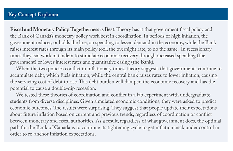
The primary policy conclusion from our experimental findings is that people do not exhibit sufficiently forward looking behaviour for expectations of future policy conflict to matter. People respond to the recent state of the economy and not on how fiscal and monetary authorities will react at some future moment in time. In other words, participants use some form of historical information to formulate their expectations, with the large majority of them using historical trends to forecast inflation and the output gap (between actual and potential output).
These findings have implications for both governments and the Bank of Canada. Ideally, with the Bank firmly in a tightening cycle to get inflation under control, governments would contribute to this fight by not adding new spending. This would help achieve those necessary results. However, should this not be the path fiscal authorities choose, while conflict might make things harder, our results suggest that the optimal path for the Bank of Canada is to continue its tightening cycle to get inflation back under control in order to re-anchor inflation expectations.
The authors thank Rosalie Wyonch, William Robson, Alexandre Laurin, Steve Ambler, Pierre Duguay, David Laidler, Angelo Melino, Nick Pantaleo, Mark Zelmer and anonymous reviewers for comments on an earlier draft. The authors retain responsibility for any errors and the views expressed.
Introduction
Central banks and governments can, and often do, act in coordination with one another to achieve common macroeconomic objectives.
An example of such coordination occurred at the start of the pandemic crisis, when monetary and fiscal authorities across multiple jurisdictions aligned their policy tools in an attempt to stabilize economies facing unprecedented lockdowns. Here in Canada, the Governor of the Bank of Canada, the Minister of Finance, and the Superintendent of Financial Institutions announced a series of coordinated measures in March 2020, in order to prevent an economic crisis from turning into a full-blown financial crisis. Despite a short and sharp drop in economic growth in the first half of 2020, these coordinated policies were broadly a success.
However, a combination of continued fiscal stimulus, unforeseen supply-side issues, e.g., the war in Ukraine, and monetary policy that was slow to tighten, have forced the central bank to turn its attention to fighting inflation, the likes of which we haven’t seen since the early 1980s. The Bank has responded by hiking the overnight rate 325 basis points since March 2022. Fiscal policy has been more mixed in its response, on the one hand shrinking the projected budget deficit – buoyed by higher tax revenue as a result of high inflation – and, on the other, using this windfall to add $11.3 billion in new spending.
If the mix of fiscal and monetary policy persists beyond what can be plausibly explainable, there is a risk that the public may come to doubt the credibility of the government’s fiscal framework and its commitment to long-run debt sustainability. Fiscal policy would then be fundamentally incompatible with the Bank of Canada’s inflation targeting mandate.
In this paper, we consider how expectations about this type of conflict affect outcomes for economic growth and inflation. Economic theory (see, for example, Bianchi and Melosi 2019) predicts that central banks and governments can achieve desired outcomes if their fiscal and monetary policies are coordinated rather than in conflict. These conclusions stem, to a large extent, from the assumption that people/agents in the economy form forward-looking, rational expectations. We use an experimental lab setting to test these assumptions and predictions.
The primary policy conclusion from our experimental findings is that people do not exhibit sufficiently forward-looking behaviour for expectations of future policy conflict to matter.
In other words, acting quickly and decisively, and seeing results, is critical for economic stability. This finding is generalizable, both in the current context, and looking ahead to future periods of economic uncertainty.
Motivation
The onset of the pandemic saw a high degree of coordination between our monetary and fiscal authorities. Facing an unprecedented economic lockdown and recession, the Bank of Canada lowered the overnight rate by 50 basis points to 1.25 percent on March 4. That was an extremely rare break from the pattern over the last two decades of 25 basis point moves. On March 11, the federal government jumped in with a $1 billion spending package. However, both sides, along with the Office of the Superintendent of Financial Institutions (OSFI), realized quickly that this support would be insufficient. On March 13, the Bank announced a surprise inter-meeting
This was just the beginning of measures by the Bank of Canada and federal government. The Bank would begin its first foray into quantitative easing (unlike the Federal Reserve, the Bank did not use quantitative easing during the 2008 global financial crisis). In addition, it moved beyond sovereign debt (federal government treasury bills and bonds) and purchased provincial government and private-sector debt. The result: assets on the Bank of Canada’s books grew from $120 billion in March of 2020 to a peak of $575 billion in early 2021.
At least as it pertains to the first part of the crisis, these programs demonstrated the importance of acting quickly and decisively in a coordinated fashion (see, for example, Ambler and Kronick 2020). Liquidity access improved immensely after worrying spikes in spreads and borrowing costs for even the safest asset, i.e., Government of Canada debt. Further, in many instances, these programs had a much lower uptake than expected, e.g., provincial debt programs, which was an indication of the importance of the Bank simply announcing that it stood ready to make these purchases. And, lastly, their use declined fairly quickly. For example, the Bankers’ Acceptance Purchase Facility had no demand by the end of July 2020.
At the same time that the Bank was pumping liquidity into the system to prevent an economic crisis turning into a financial one, the federal government was adding to its fiscal support, primarily through the Canada Emergency Response Benefit (CERB) and the Canada Emergency Wage Subsidy (CEWS). The former was geared at those workers who were directly impacted by the pandemic lockdowns, and paid $500 a week to those eligible. The latter evolved over time in terms of who was eligible and how a business qualified, but in principle, the concept was the same: employers that lost a certain percentage of their revenue qualified for a wage subsidy.
The Canadian economy, after the two largest monthly declines in GDP on record in March and April of 2020, began a rebound in May that has continued ever since, though with bumps along
the way.
However, since April 2021, inflation in Canada has far exceeded the top end of the Bank of Canada’s inflation target range (1-3 percent), which reflects the Bank being slow off the mark in tightening monetary policy, alongside continued fiscal stimulus. As the Bank tightens monetary policy - to the tune of 325 basis points since March, fiscal policy has been mixed, on the one hand having its shortfall shrink as a result of higher tax revenue from higher inflation, while on the other hand spending some of that windfall on new government spending.
In this paper, our goal is to understand how these fiscal and monetary authority interactions – be they coordination and/or conflict – at different points in the cycle (e.g., recession/recovery), affect macroeconomic expectations, and, as a result, macroeconomic outcomes.
Predictions under Rational Expectations
We focus our study on a scenario where an economy is in the middle of a recession with the expectation that it is headed for an economic recovery with excess demand. At such a point, there are essentially four paths forward:
- A monetary-led coordinated scenario – where the central bank, once in excess demand, actively works to bring inflation back to target by raising the interest rate, and where the government commits to stabilizing the debt-to-GDP ratio so as not to further stimulate demand, which would place further upward pressure on prices;
- A fiscally led coordinated path – where the government does not stabilize the debt-to-GDP ratio, or, at least, continues to further stimulate economic growth, and where the central bank takes a “passive” stance on inflation, resulting in inflation remaining above target and thus helping with the higher debt load;
- A conflict scenario with fiscally led resolution – where the government initially pursues an expansionary fiscal policy despite the economic recovery moving into excess demand, while the central bank pursues a more aggressive contractionary monetary policy to tame price increases, and ultimately the government “wins” with the central bank taking a more passive stance to inflation; and
- A conflict with monetary-led resolution – where, again, the government initially pursues an expansionary fiscal policy in the economic recovery while the central bank pursues a more aggressive contractionary monetary policy, but this time the central bank “wins” and the government is forced to rein in its spending.
Setting the conflict as temporary is necessary in order to generate a stable equilibrium. Without defining the end of the conflict period, inflation, output, and debt set out on an explosive path. Our experiments test whether this stability through defining an end to the conflict holds in practice.
The anticipation of policy conflict after a recession is predicted to generate deeper and more severe recessions during the economic downturn (Bianchi and Melosi 2019). If governments continue to accumulate debt, which fuels inflation, while the central bank raises rates to lower inflation, the servicing cost of debt will rise. This debt burden will dampen the economic recovery and has the potential to cause a double-dip recession. If people are sufficiently forward looking in the midst of a recession, they will form more pessimistic expectations as they anticipate the consequences of policy conflict. During an economic recovery, households and businesses, aware of the policy conflict, expect even higher inflation, leading to actual higher inflation, which negatively affects central bank credibility.
Under the coordinated scenarios, because rational agents anticipate that the monetary and fiscal authorities will work together, the recession is less severe, and the recovery is stronger, happening at a quicker pace. Fiscally led coordinated scenarios typically lead to stronger recoveries (as measured by output) with the additional boost from government spending, but at the expense of inflation above target.
In these economic models, coordination is key for dealing with business cycle fluctuations. Crucially, the typical economic models that make these predictions depend on the assumption that people are forward looking; that is, they anticipate the actions of the central bank and the government in the future, and update their inflation expectations accordingly in the present. We ask whether this is true: are people as forward looking as models assume? If they are not – or, at least, not as much as we think – we ask if it is most important for authorities, whether fiscal or monetary, to act quickly, and to get inflation (and other important macroeconomic variables) under control as fast as possible regardless of what the other is doing.
Experimental Design
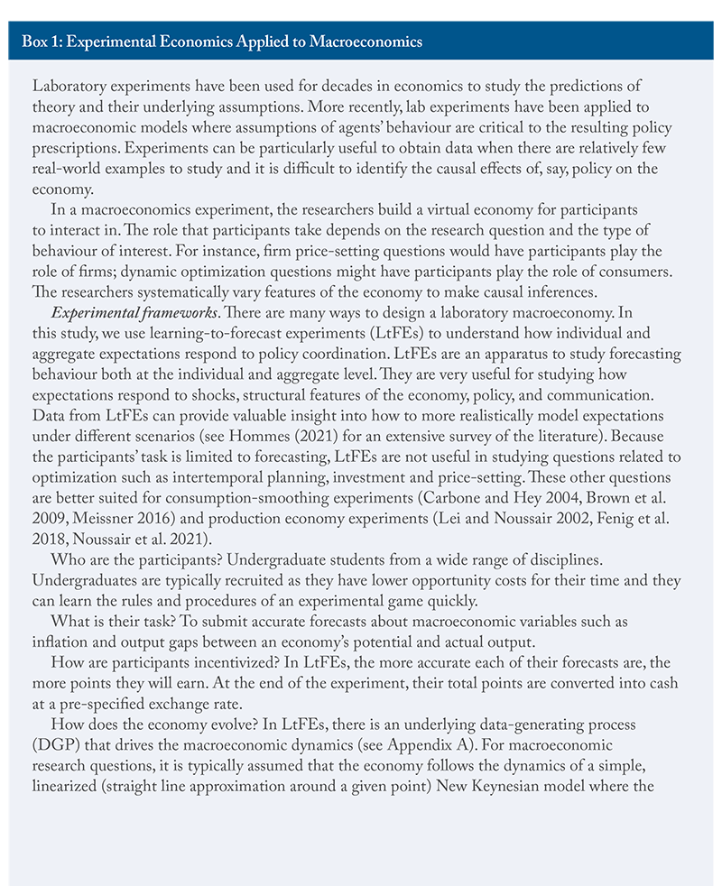
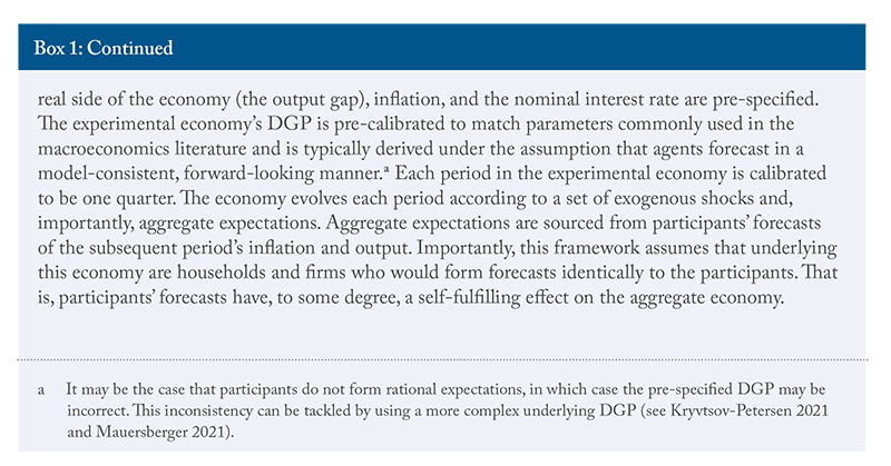
To test this economic model of policy conflict and coordination, we designed a lab experiment where participants, consisting of undergraduate students from diverse disciplines, interacted in a simulation economy and were asked to make predictions about future macroeconomic outcomes, including inflation. Lab experiments are becoming more and more common in macroeconomics as the underlying assumptions of many economic models have been called into question. Box 1 describes how a macroeconomy can be implemented in the lab using Learning-to-Forecast Experiments (LtFEs), first developed by Marimon and Sunder (1994) and extended for macroeconomic questions by Adam (2007). By using a simplified model economy, we can see how people form beliefs and make decisions based on the information they are presented with, and whether they behave in the same way that economic theory would expect them to.
Participants were tasked with playing the role of professional forecasters and would be incentivized to make forecasts about inflation and output in a simulated LtFE economy. Appendix A provides quantitative details of the experimental economy. In our economy, participants’ forecasts and exogenous (external) shocks to aggregate demand feed into the economy’s data-generating process (DGP) and drive aggregate dynamics.
During the instruction phase, we provided participants with complete information about the structure of the economy, including detailed information about the government debt level, the tax rate, and the interest rate to inform their decisions. They were informed that they would interact in an economy for 30 rounds, which would consist of two or three phases of unspecified length. In Phase 1 (which lasted 10 rounds), the economy was in a recessionary, low-demand state, and both the government and the central bank would be engaging in expansionary fiscal and monetary policy in order to stimulate demand. In the remaining phases, the economy would return to the high-demand state. Depending on the treatment, the monetary and fiscal authorities entered the recovery phase(s) either coordinating their policy decisions or in conflict. For the remaining 20 rounds, phases 2 (11-20 in conflict or to 30 in coordination) and 3 (21-30 only in conflict), as the economy returned to a high-demand state, participants would find themselves in one of the four scenarios we described above: either a monetary-led coordinated recovery; fiscally led coordinated recovery; a conflict recovery with a fiscally led resolution; or a conflict recovery with a monetary-led solution.
In the (coordinated) monetary policy Led (MP Led) treatment, we informed participants that:
“When consumer demand eventually recovers, output and inflation will begin to rise. The government and central bank will follow a coordinated strategy to simultaneously reduce debt and inflation. The government will reduce its spending and collect more taxes to reduce its debt level, i.e., run fiscal surpluses. The central bank will begin to raise the interest
rate more than one-for-one with inflation.”
During the economic recovery, participants were told that taxes and the interest rate will be calculated as follows:
Taxt = 0.966 Taxt-1 + 0.009 Outputt
+ 0.002 Debt Levelt-1
Interest Ratet = 0.657 Interest Ratet-1
+ 1.2 (Inflationt – 0) + 0.09 (Outputt – 0)
Increasing the amount of tax collected will reduce the government’s debt level. Raising the interest rate will make it more expensive for households and firms to borrow, thereby reducing demand and indirectly reducing inflation. Higher interest rates also cause the government’s debt level to rise. This will, in turn, lead to higher taxes as the government aims to stabilize its debt level.
In the (coordinated) fiscal policy led (FP Led) treatment, we informed participants that:
“When consumer demand eventually recovers, output and inflation will begin to rise. The government and central bank will continue to follow a coordinated strategy to keep the economy growing. The government will reduce its spending but will continue to ignore its debt level when deciding how much to collect in taxes. The central bank will continue to respond weakly to any changes in inflation.”
As above, we informed participants on how the path for taxes and the interest rate would be calculated:
Taxt = 0.65 Taxt-1 + 0.098 Outputt
Interest Ratet = 0.657 Interest Ratet-1 + 0.236 (Inflationt – 0) + 0.091 (Outputt – 0)
As output and inflation improve, the government will spend less. This, together with growing inflation and relatively low interest rates, will help the government to reduce its debt level.
In the two conflict treatments, participants were informed that:
“When consumer demand eventually recovers, output and inflation will begin to rise. The government and central bank will face a conflict in how to approach the recovery. The government will reduce its spending but will continue to ignore its debt level when deciding how much to collect in taxes. The central bank, on the other hand, will begin to raise the interest rate more than one-for-one with inflation.”
Taxes and the interest rate were calculated as follows:
Taxt = 0.65 Taxt-1 + 0.098 Outputt
Interest Ratet = 2 (Inflationt – 0) + 0.265 (Outputt – 0)
By increasing the interest rate, the central bank aims to reduce inflation. The combination of lower inflation and higher borrowing costs, exacerbates the government’s debt level.
In the conflict then monetary policy led (ConflictMP) treatment, participants were told that eventually the conflict would end and the government would begin taxing more to manage its debt level.
Participants were informed that once the conflict ended, taxes collected by the government would be given by:
Taxt = 0.966 Taxt-1 + 0.009 Outputt + 0.002 Debt Levelt-1
Participants were also told that the central bank would continue to aggressively adjust its interest rate to keep inflation and output gap close to target, and interest rates would follow the following path:
Interest Ratet = 0.657 Interest Ratet-1 + 1.2 (Inflationt – 0) + 0.091 (Outputt – 0)
In the conflict then fiscal policy led (ConflictFP) treatment, participants were told that eventually the conflict would end and the central bank would lessen its response to inflation. The government would continue to ignore its debt level when deciding how much to collect in taxes. The only change once the conflict ended was to the central bank’s interest rate response to inflation:
Interest Ratet = 0.657 Interest Ratet-1 + 0.236 (Inflationt – 0) + 0.091 (Outputt – 0)
Relatively lower interest rates, together with higher inflation, will help the government to reduce its debt level.
We provided participants with complete information about the economy’s structure, including a full quantitative model that clarified the relative importance of different variables in driving inflation and the output gap (see Appendix A). Importantly, they had complete information about the economy’s structure, the monetary and fiscal authorities’ policy rules, and that the economy would go through two or three phases. Participants did not know when the economy would move from the low to the high state, nor did they know when the conflict would end (in the conflict treatments). The experimental economy is directly modeled on the theoretical framework of Binachi and Melosi (2019). While monetary policy directly influences aggregate demand, fiscal policy – namely, the government’s debt level – can only impact the economy through its effect on expectations.
Under the assumption that the public is forward looking, the conflict scenarios are predicted to produce short-run economic instability as the government’s debt grows rapidly in response to the central bank’s aggressive response to inflation.
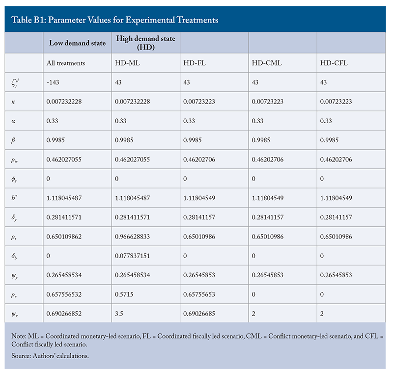
Appendix B has the parameter values used for each treatment.
Lab Results
In this section, we ask whether our experiments confirm the following conclusions from standard economic theory:
- the recessions are deeper and more severe under policy conflict;
- the recovery is stronger and happens more quickly under policy coordination;
- recoveries are stronger in coordination – whether it be right after the low demand state or after conflict – under fiscally led scenarios, but at the expense of having inflation above target.
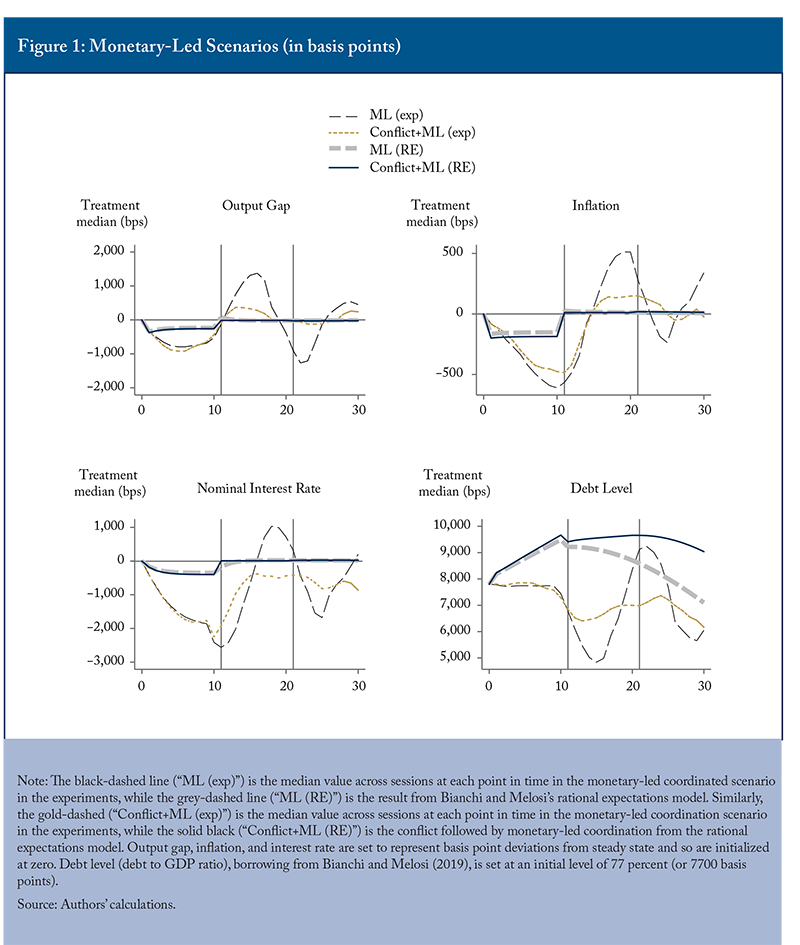
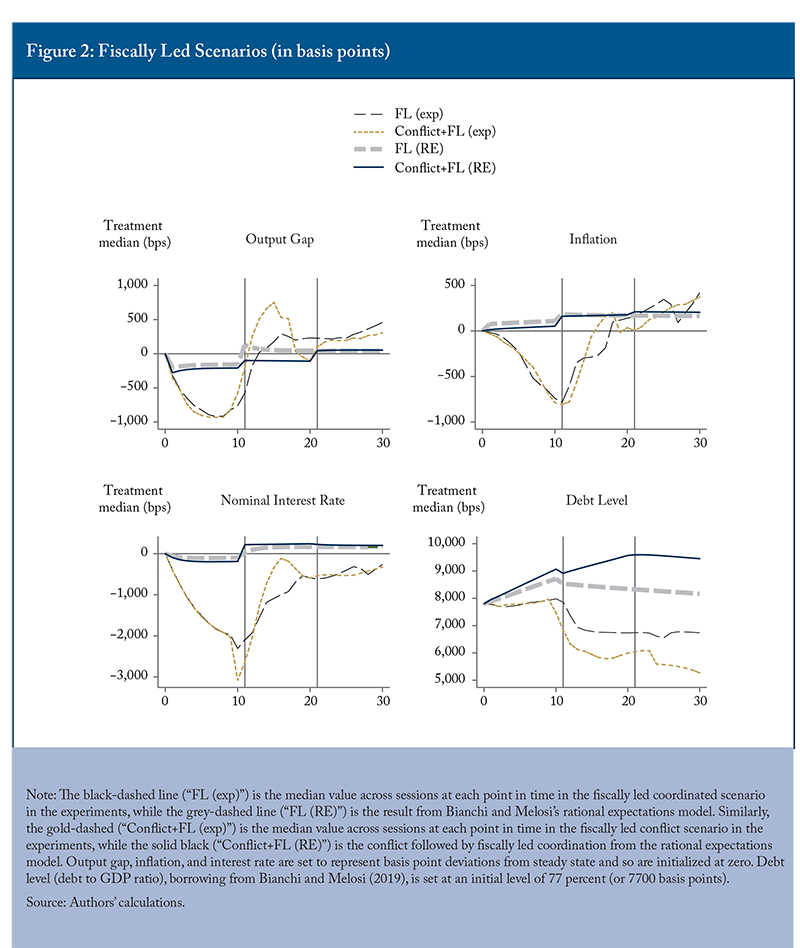
Figures 1 and 2 show the results in both theory and in the lab under both the monetary (coordinated and conflict) and fiscal (coordinated and conflict) scenarios, respectively. The lines for the experiment (black-dashed lines for coordination and gold-dashed lines for conflict) represent median values across treatments. The gray-dashed (coordinated) and black solid (conflict) line are the results from running the Bianchi and Melosi (2019) model using the parameters in Appendix B.
What is most important in interpreting these graphs is not the quantities themselves, but the directions relative to standard economic theory and the differences when comparing different scenarios.
Prediction 1: Initial Recessions are Deeper in Policy Conflict Situations
Finding 1: Lab results predict recessions are NOT deeper in policy conflict situations.
Our first testable hypothesis is that the initial recessions are deeper in policy conflict situations than they are in coordination situations both in the monetary-led and fiscally led scenarios.
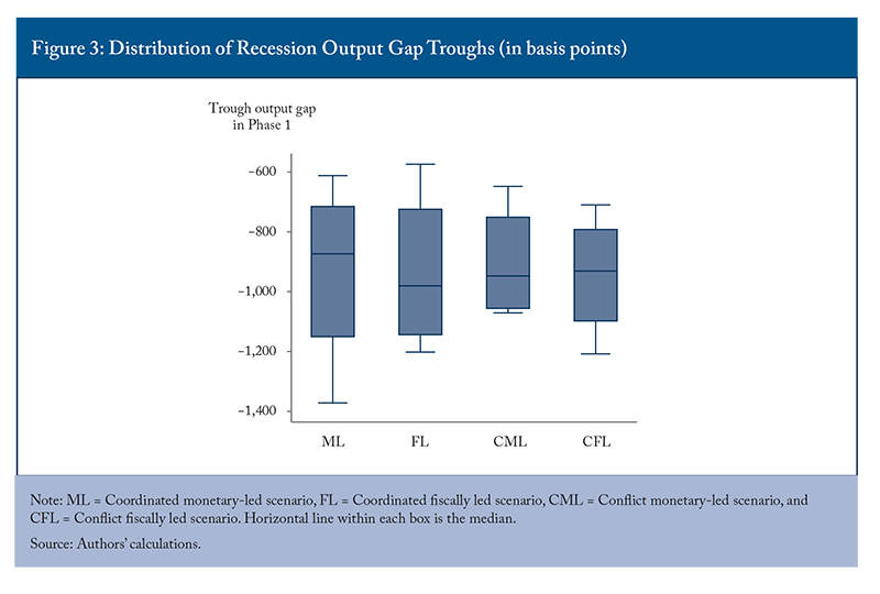
We do not find support for this hypothesis. Specifically, the median results during the recession (phase 1) when we compare coordination versus conflict in each of the monetary and fiscally led scenarios are almost indistinguishable (Figures 1 and 2). Future policy mix makes little difference during the recession phase.
Putting numbers to this finding, in the monetary policy scenarios, the average output gap trough is -945 basis points when there is coordination and -934 basis points in conflict (Figure 3). Similarly, in the fiscal policy scenarios, the average output gaps are -903 basis points under coordination and -933 basis points in conflict. Comparing the two types of scenarios, we find that coordination and conflict scenarios experience comparable troughs during the recession phase of the experiment.
Prediction 2: Recovery is Stronger and Faster with Policy Coordination
Finding 2: Lab results suggest recovery is strongest and fastest under monetary-led policy coordination
Our second testable hypothesis was that the output gap rebound when the economy returned to normal was greater with coordination – regardless of being fiscal versus monetary-led – as was the speed with which the recovery occurred.
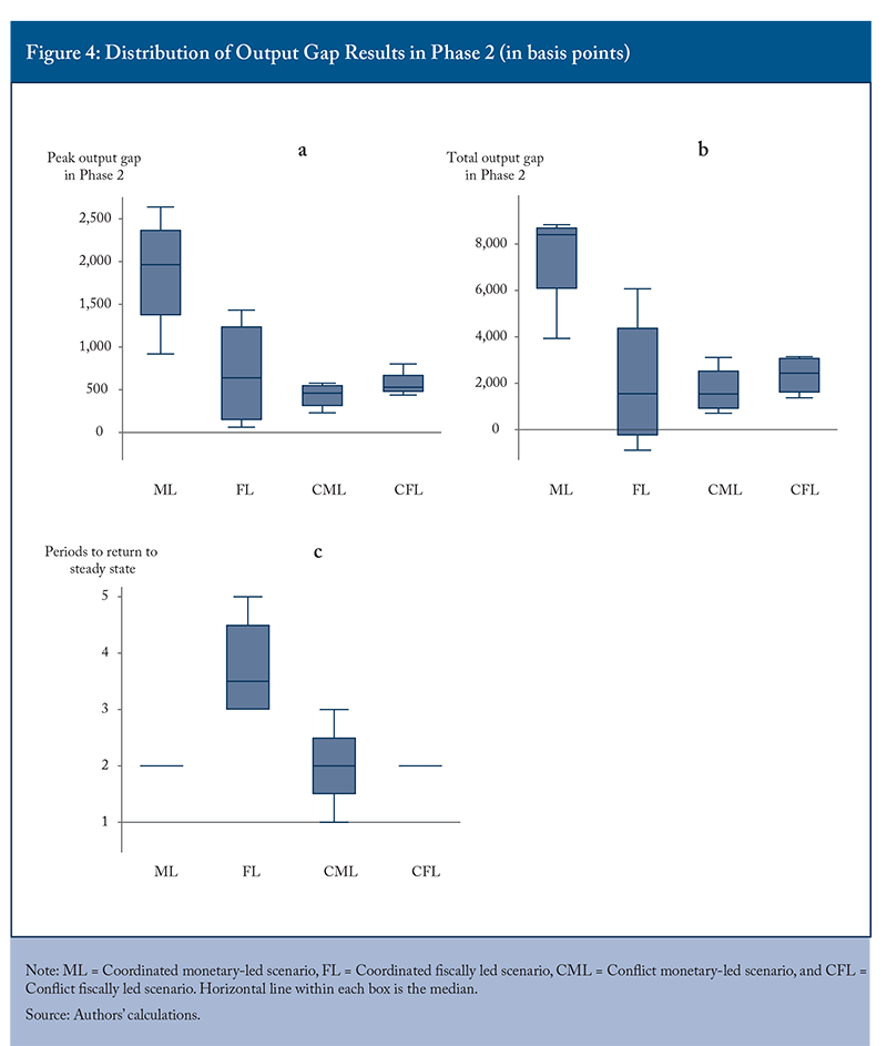
Our experiments provide mixed support for these predictions. On the one hand, the peak of the recovery is stronger in coordination scenarios. Figure 4 panel (a) shows the distribution of the peaks of the output gaps in phase 2.
The results are also mixed when using an alternative measure of the size of the recovery – the total output gap – in phase 2. Panel (b) shows the distribution of the total output gaps across sessions for each treatment. On this metric, while the average total output gap is largest in the coordinated monetary-led scenario (7,392 basis points), it is followed not by fiscally led coordinated scenario but by the fiscally led conflict scenario (2,347 basis points).
In terms of speed of recovery, panel (c) in Figure 4 presents the number of periods before the economy in a particular session returns back to the steady state. The average session in each of monetary-led coordination and both conflict scenarios takes two periods to return to its pre-recession state. The coordinated fiscally led scenario is more sluggish, however, taking an average of 3.75 periods. Taken together, these results suggest that recovery is not ubiquitously faster in coordinated scenarios.
Prediction 3: During the Recovery – Regardless of Coordination/Conflict – Fiscally Led Scenarios Lead to Stronger Output Recoveries, but at the Expense of Inflation Well Above Target
Finding 3: Lab results indicate that economic recovery is strongest under monetary-led coordination with limited inflation. Fiscal leadership does not necessarily imply worse inflation.
Our last testable hypothesis is that the recovery in the policy coordination scenarios is stronger when the fiscal authority eventually leads, though gains under fiscally led scenarios come at the expense of inflation well above target. Under the monetary-led scenarios, inflation is essentially at target.
Our experiments provide little support for these predictions. When there is clear coordinated leadership immediately following the recession, the economic recovery in phase 2 is significantly stronger under monetary-led coordination than fiscally led coordination (as we saw above in Figure 4 panel a)).
Following the conflict scenarios, phase 3 economic recovery and inflation are on average stronger under fiscally led than monetary-led scenarios. Peak output (inflation) under fiscally led is 1,698 bps (698 bps), while only 388 bps (111 bps) under monetary-led. However, both treatments exhibit notable variance across sessions in inflation and output, and, as a result, the differences across regimes on the whole are not statistically significant.
Policy Implications
What does it mean that the lab results differ so markedly from what we expected based on economic theory? And, what does it mean in practice for Canada’s monetary and fiscal policy.
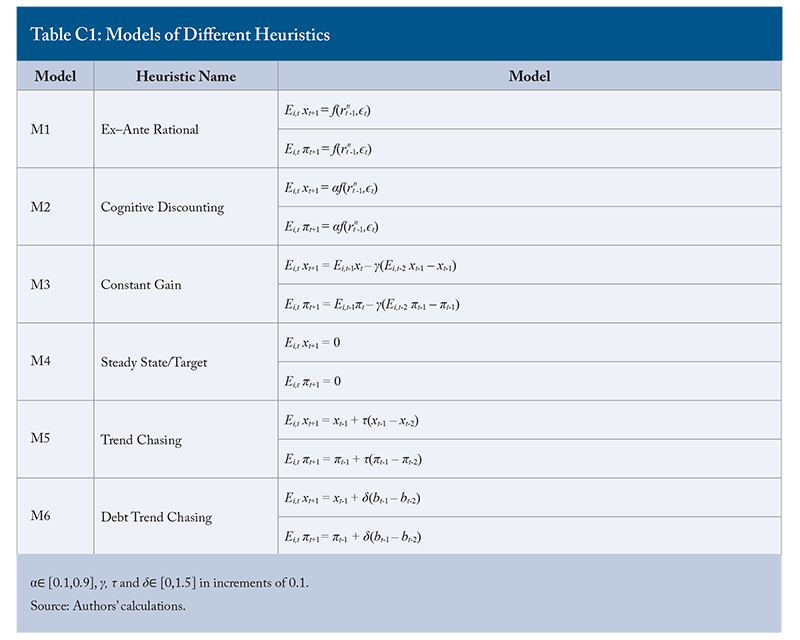
To help us answer these questions, we use the experimental data from participants’ forecasts to determine how they form their expectations. We categorize these mental shortcuts into types and assign a type to each participant that best fits their forecasting behaviour. Table C1 in Appendix C summarizes all the types (heuristics in economists’ terms) we have considered in mathematical terms.
The simplest deviation from rational expectations is called cognitive discounting (Gabaix 2020), where households/businesses discount variables far into the future to a larger degree than we expect.
We also consider backward-looking types in which the formation of expectations is history driven, e.g., constant-gain learning (see, for example, Evans and Honkapohja 2012 and Milani 2008).
Lastly, we look at two trend-chasing expectations:
- expectations of next period’s output/inflation is based on last period’s output/inflation, though with the addition of a trend-chasing parameter that gives weight to how last period’s output/inflation evolved from output/inflation the period before that; and
- another form of trend-chasing, one focused on government debt instead of output/inflation.
We determine the forecasting type for each participant that best fits their forecasting behavior during each phase of the experiment (Figure 5 for inflation forecasts and Figure 6 for output forecasts).
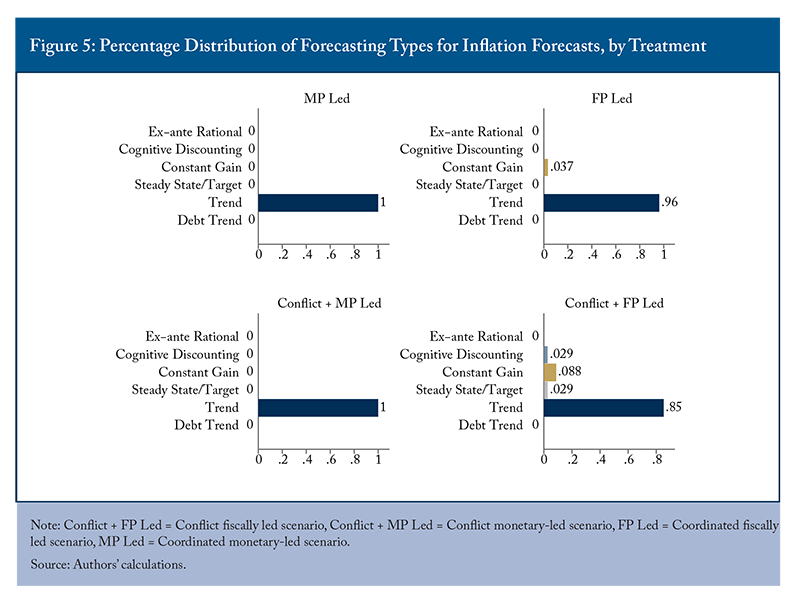
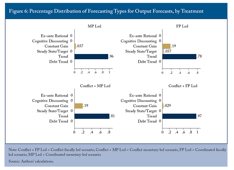
We find that economic fundamentals and the government’s debt do not weigh significantly in their forecasts. Rather, participants use some form of historical information to formulate their expectations. The large majority of them use historical trends to forecast inflation and the output gap. There is a wide range within each treatment in the degree of trend-extrapolation, but not across treatments. That is, the treatments themselves do not significantly change the way in which people forecast.
When people mostly extrapolate trends, updating their expectations based on what has happened in the past, it matters how the central bank and government individually set policy following an economic downturn. If people are likely to form backward looking expectations, it is important for the authorities to maintain economic stability. The conflict between policymakers means the central bank takes an even more aggressive stance on inflation. This works well to manage inflation and, in turn, inflation expectations. By being relatively relaxed about inflation in the monetary-led regime, we see that inflation can become more volatile and expectations can become significantly unanchored. The importance of aggressive monetary policy responses to manage inflation expectations has also been documented by Kryvtsov and Petersen (2015) and Pfajfar and Žakelj (2018).
Conclusions
Canadians are in the midst of inflation the likes of which we haven’t seen in 40 years, and as prices continue to rise, inflation is becoming a salient issue for more and more people. Our lab results suggest that people update their expectations about future inflation based on current and previous trends, regardless of coordination or conflict between monetary and fiscal authorities.
There are implications for both governments and the Bank of Canada. Ideally, with the Bank firmly in a tightening cycle to get inflation under control, governments would contribute to this fight by not adding new spending. This would help achieve those necessary results. However, should this not be the path fiscal authorities choose, while conflict might make things harder, our results suggest that the optimal path for the Bank of Canada is to continue its tightening cycle to get inflation back under control in order to re-anchor inflation expectations.
The prevalence of backward-looking expectations also has important implications for the choice of monetary policy frameworks more generally. Many central banks, including the Bank of Canada, have recently entertained introducing make-up strategies into their frameworks (e.g., allowing for more inflation to compensate for recently low inflation and vice versa). These strategies create better anchored expectations if the public is forward looking and anticipates the make-up down the road. Our results demonstrate that such strategies may not work as intended.
Appendix A: Macroeconomic Dynamics
The structure of the experimental macroeconomy comes from a linearized version of the model developed in Bianchi and Melosi (2019). The macroeconomy can be described by the following system of equations:

Equation 1 describes how the economy’s output gap evolves in response to aggregate expectations of period t+1 output gap, Et xt+1, and the real interest rate, Rt – Et πt+1, where Rt is the central bank’s policy rate and Et πt+1 refers to the aggregate expectation of period t+1 inflation. Equation 2 is the New Keynesian Phillips curve and describes inflation driven by aggregate expectations of inflation and the output gap. κ governs the pass-through of monetary policy and other factors that affect aggregate demand to inflation.
The policy rule of the central bank is given by:

Equation 3 describes the reaction function of the central bank, where ψπ governs the response to deviations of inflation from target and ψy the response to deviations of output from target. The parameter ρR denotes the degree of persistence in the central bank’s policy rate.
On the fiscal side, the government’s tax rate evolves according to the following equation:

where bt, the government’s real debt level, is given by

Equation 4 says that the central bank increases its taxes as the output gap and the level of past real debt, bt-1 grow larger. The parameter ρτ denotes the degree of persistence in the government’s tax rate.
Equation 5 describes the evolution of real government debt. Real government debt increases as the output gap contracts, inflation is low, the government taxes less, and nominal interest rates rise.
The exogenous demand shock, ζtd, follows a two-state Markov process. In the low state, ζtd = -143 bps. The probability that the economy remains in the low state in the next period is 0.94. In the high state, ζtd = 43 bps. The probability that the economy remains in the high state in the next period is 0.99.
We close the model by specifying the aggregate expectations that are key to driving aggregate dynamics. Aggregate expectations are elicited by our experimental participants. Each period t, participant i forms expectations about the next period’s output gap, Ei,t xt+1, and inflation, Ei,t πt+1. The median forecast of each variable is used as the aggregate forecast and fed into the economy’s data-generating process to determine the macroeconomic dynamics.
Appendix B: Parameter Values
We take the bulk of the parameter values directly from Bianchi and Melosi (2019), making minor adjustments we felt better suited the Canadian economy and the reaction function of the Bank of Canada (Table B1).
We note that the persistence parameter for the central bank, labelled ρr, is different under coordination and conflict. The intuition is that whether inflation causes an increase or decrease in real debt comes down to how aggressive the central bank reaction function with respect to inflation above target is – the more aggressive it is, the more likely real debt will increase. To generate the double dip recession under conflict in this model, debt servicing costs for the government must go up, which requires a secondary increase in interest rates from the higher inflation the government needs to pay down their increased debt load (the higher debt/higher inflation/higher interest rate spiral). To get these higher interest rates, we need the central bank to respond aggressively to inflation above target, which we get by removing any persistence in the Taylor rule.
Because we then need this persistence parameter to be positive in coordination, this also affects the parameters we need in the Taylor Rule equation to generate the greater than one-for-one reaction of interest rates to inflation under active monetary policy.
We incentivize participants to forecast accurately by awarding them points according to the following scoring rule:

At the end of each period t, subjects would receive points based on the forecast accuracy of their period t-1 forecasts about period t inflation and output gap. For every 100 basis point error participants made for each of their two forecasts, their score would drop by one-half. Points were exchanged for Canadian dollars at an exchange rate of $1.25 per point.
Appendix C: Forecasting Types
We note that for some types, such as Cognitive Discounting, Constant Gain, and Trend-Chasing, we consider a wide range of parameterizations. The cognitive discounting parameter α can take values in the range of [0.1,0.9]. The constant gain parameter γ and trend-chasing parameter τ are in the range of [0,1.5]. We consider values of these parameters from these ranges with an increment of 0.1.
References
Adam, K. 2007. “Experimental Evidence on the Persistence of Output and Inflation.” The Economic Journal, 117(520): 603-636.
Ambler, S. and Kronick J. 2020. “Canadian Monetary Policy in the Time of COVID-19.” E-Brief 307. Toronto: C.D. Howe Institute. October.
Assenza, T., Heemeijer, P., Hommes, C. H., and Massaro, D. 2013. “Individual Expectations and Aggregate Macro Behavior.” Tinbergen Institute Discussion Papers 13-016/II, Tinbergen Institute.
Bianchi F. and Melosi L. 2019. “The Dire Effects of the Lack of Monetary and Fiscal Coordination.” Journal of Monetary Economics. 104:. 1-22.
Brown, A. L., Chua, Z. E., and Camerer, C. F. 2009. Learning and Visceral Temptation in Dynamic Saving Experiments. The Quarterly Journal of Economics, 124(1): 197-231.
Carbone, E., and Hey, J. D. 2004. “The Effect of Unemployment on Consumption: An Experimental Analysis.” The Economic Journal, 114(497): 660-683.
Clarida, R., Gali,J., and Gertler, M. 2000.. “Monetary Policy Rules and Macroeconomic Stability: Evidence and Some Theory.” Quarterly Journal of Economics. Volume 115(1): 147-180. February.
Cole, S. J., and Milani, F. 2021. “Heterogeneity in Individual Expectations, Sentiment, and Constant-gain Learning.” Journal of Economic Behavior & Organization, 188: 627-650.
Cornand, C., and M’baye, C. K. 2018. “Does Inflation Targeting Matter? An Experimental Investigation.” Macroeconomic Dynamics, 22(2): 362-401.
Corsetti G.,. Dedola, L. Jarocinski, M. Mackowiak, B., and Schmidt, S. (2019). “Macroeconomic Stabilization, Monetary-Fiscal Interactions, and Europe’s Monetary Union.” European Journal of Political Economy. 57: 22-33. March.
Evans, G. W., and Honkapohja, S. 2012. Learning and Expectations in Macroeconomics. Princeton University Press.
Fenig, G., Mileva, M., and Petersen, L. 2018. “Deflating Asset Price Bubbles with Leverage Constraints and Monetary Policy.” Journal of Economic Behavior & Organization, 155: 1-27.
Gabaix, X. 2020. “A Behavioral New Keynesian Model.” American Economic Review, 110(8): 2271-2327.
Gali J. 2015. Monetary Policy, Inflation, and the Business Cycle. Princeton: Princeton University Press.
Gaspar, V., Smets, F., and Vestin, D. 2006. “Adaptive Learning, Persistence, and Optimal Monetary Policy.” Journal of the European Economic Association, 4(2-3): 376-385.
Hommes, C. 2021. “Behavioral and Experimental Macroeconomics and Policy Analysis: A Complex Systems Approach.” Journal of Economic Literature, 59(1): 149-219.
Lei, V., and Noussair, C. N. 2002. “An Experimental Test of an Optimal Growth Model.” American Economic Review, 92(3): 549-570.
Kostyshyna, O., Petersen, L., and Yang, J. 2022. A Horse Race of Monetary Policy Regimes: An Experimental Investigation. (No. w30530). National Bureau of Economic Research.
Kryvtsov, O., and Petersen, L. 2013. Expectations and Monetary Policy: Experimental Evidence. (No. 2013-44). Bank of Canada.
Marimon, R., and Sunder, S. 1994. “Expectations and Learning Under Alternative Monetary Regimes: An Experimental Approach.” Economic Theory, 4(1): 131-162.
Meissner, T. 2016. “Intertemporal Consumption and Debt Aversion: An Experimental Study.” Experimental Economics, 19(2): 281-298.
Milani, F. 2008. “Learning, Monetary Policy Rules, and Macroeconomic Stability.” Journal of Economic Dynamics and Control, 32(10): 3148-3165.
Noussair, C. N., Pfajfar, D., and Zsiros, J. 2021. “Frictions in an Experimental Dynamic Stochastic General Equilibrium Economy.” Journal of Money, Credit and Banking, 53(2-3): 555-587.
Petersen, L. 2014. “Forecast Error Information and Heterogeneous Expectations in Learning-to-Forecast Macroeconomic Experiments.” Experiments in Macroeconomics. Emerald Group Publishing Limited.
Pfajfar, D., and Žakelj, B. 2014. “Experimental Evidence on Inflation Expectation Formation.” Journal of Economic Dynamics and Control, 44: 147-168.
Pfajfar, D., and Žakelj, B. 2018. “Inflation Expectations and Monetary Policy Design: Evidence from the Laboratory.” Macroeconomic Dynamics, 22(4), 1035-1075.
Woodford M. 2003. Interest and Prices: Foundations of a Theory of Monetary Policy. Princeton, New Jersey: Princeton University Press.


