Money Talks: The Old, New Tool for Predicting Inflation

The Study In Brief

With rising inflation top-of-mind for Canadians, a major question is: Can we predict its future? This Commentary shows that growth in the money supply is a useful predictor of inflation, and examines why and when.

Since the early 1990s, the Bank of Canada has pursued a successful inflation-targeting strategy. With inflation, and inflation expectations, safely anchored in the Bank’s target 1-3 percent band, tracking the growth of money supply in the economy as an aid in forecasting inflation fell out of fashion. In this Commentary, we examine both the short- and long-run relationship between money supply growth and inflation and find both matter for monetary policy.

Our results have important implications for the analysis of monetary policy and inflation during the current pandemic period. Canadian money supply grew in 2020 and 2021 at unprecedentedly high rates, inflation is now nearly 6 percentage points above the 2 percent target, and measures of inflation expectations show that inflation is not expected to return to target within the Bank of Canada’s usual planning horizon of six to eight quarters.

This paper answers two questions:

• Is there still a long-run relationship between monetary aggregates and inflation despite the disappearance of the short-run relationship starting in the 1980s?
• If the main (but not only) explanation for the disappearance of the short-run relationship is the fact that the target itself is the best predictor of inflation in an inflation-targeting regime, then when the regime is not operating as expected does the short-run relationship return?

We find that the long-run relationship does, indeed, continue to hold, and did so even during the inflation-targeting era. We also find that keeping track of money does often reduce the margin of error in forecasting inflation when the latter deviates substantially away from target, as it does today.

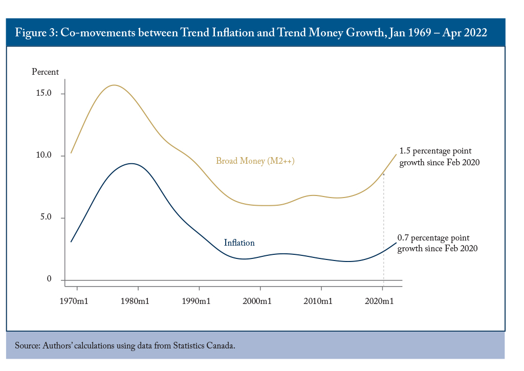
With “trend” money growth (screening out short-term fluctuations over time) now 1.5 percentage points above where its value was prior to the pandemic, and “trend” inflation not quite half of that, we are not done with price growth yet, meaning the Bank will have to work extra diligently to anchor inflation expectations. Accelerating its pace of quantitative tightening (QT) by reducing the oversized quantity of bonds on its balance sheet and continued forceful communications around the hikes to come should be part of this effort.

Introduction

Until the early 1980s, most economists subscribed to the notion that there was a significant positive correlation, in both the short and long runs, between monetary aggregates and inflation.

However, the short-run relationship deteriorated in the mid-1980s, and today’s central bankers pay little attention to the growth rates of monetary aggregates – which measure everything from cash and bank deposits to Canada Savings bonds, net mutual fund contributions and more (see Key Concept Explainer) – in their forecasts of inflation and when making their monetary policy decisions.

This would seem to discredit monetarismMonetarism is the school of economic thought that maintains that the money supply (the total amount of money in an economy) is the chief determinant of current dollar GDP in the short run and the price level over longer periods. See: https://www.imf.org/external/pubs/ft/fandd/2014/03/basics.htm and monetary approaches to understanding inflation and monetary policy, but we argue that this is not the case.As have several others before this paper, including, among others, Bergevin and Laidler (2010). It is merely an example of a general principle attributable to Rowe and Yetman (2002) and Otto and Voss (2014). As stated in the latter paper, “if the Bank of Canada is strictly (and successfully) targeting an inflation rate of 2 percent at a two-year horizon, then current deviations of inflation from 2 percent should be unpredictable with any information that was available to the Bank two years earlier.” This means not only that monetary aggregates should not be useful to predict inflation two years out, but neither should unemployment, the output gap (between actual and potential economic output), or the Bank of Canada’s main policy instrument, the overnight rate. In fact, only the inflation target itself should predict inflation at that horizon.

This is, of course, predicated on the central bank successfully achieving its target. As Figure 1 shows, this has not been the case of late, with headline inflation above the top end of its 1-3 percent target band since April 2021. The Bank of Canada’s recent surveys of consumer and business expectations show that inflation is not expected to return to target within the next two years. Indeed, in February 2022, consumers’ expectations for inflation over the next two years averaged more than 4.5 percent (Bank of Canada 2022, Chart 1). Among firms responding to the Business Outlook Survey, 96 percent expected inflation to average at least 2 percent over the next two years, with over half of those firms expecting inflation to remain “substantially” above 2 percent for at least two years (Bank of Canada 2022a, Charts 10 and 11).

A recent working paper by Papadia and Cadamuro (2021), looking at data from the US and the euro area, presents convincing evidence that confirms this idea. They find that a strong relationship in the data between monetary aggregates and inflation exists only in “unsettled monetary and inflationary conditions.”While there is no specific definition for unsettled conditions in Papdia and Cadamuro, for our purposes, we take it to mean any period where inflation is consistently above the top end of the 1-3 percent target band. When inflation is close to target, “there is no apparent relationship between monetary aggregates and inflation.”

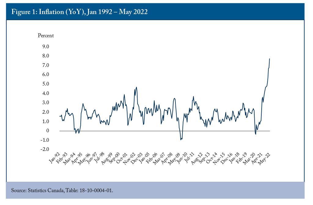
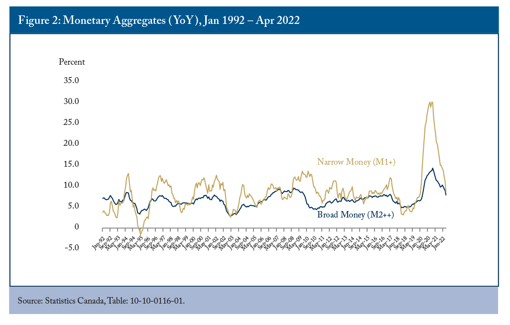
Figure 1 showed the degree of unsettled inflation, and Figure 2 does the same looking at both narrow (think cash and chequing deposits, in this case M1+) and broad (think additional retail instruments like saving deposits, in this case M2++) monetary aggregates. While the growth rates have come down since their peak, they remain elevated relative to where they have been during the inflation-targeting era.If instead we used three-month money growth rates (annualized), the sharp increase at the beginning of the pandemic would be met with a quicker fall back to more normal levels. However, it is only in the last two months (March and April 2022) where M2++ and M1+ respectively have returned, and fallen below, their pre-pandemic, average inflation-targeting era growth rates.

However, even in settled conditions there is a robust long-term relationship between monetary aggregates, “the money supply”, on the one hand, and both nominal incomePut simply, nominal income is the nation’s total annual value of goods and services including inflation. and prices on the other hand. In other words, long-run monetary neutrality – the idea that in the long run, an increase in money leads eventually to a proportional increase in nominal income – continues to hold for monetary aggregates. This has been documented in work on specific countries (see, for example, Serletis and Coustas 2019),These authors show that for the United States there is no evidence against long-run monetary neutrality for either narrow or broad monetary aggregates. as well as for larger panel studies, which take big groups of countries into consideration (see, for example, Gao et al. 2021).They show that monetary forces are still the dominant cause of movements in inflation. In their words, “the quantity theory relationships are alive and well.” (See Appendix 1 for an explanation of the quantity theory of money.). Benati (2009) finds strong evidence of long-run monetary neutrality, and Benati, Lucas, Nicolini and Weber (2021) find strong evidence, using an international data set, of a stable relationship between narrow money and income. This would imply the long-run neutrality of M1 as long as the nominal interest rate, which is the relevant opportunity cost of holding money, was stationary.

In the Canadian context, past work (see Ambler 1989) has shown that deviations from the long-run relationship between money and nominal incomeIn other words, deviations of the velocity of circulation from its long-run trend. In economics, velocity of circulation is defined as the number of times one dollar is spent to buy goods and services per unit of time. have significant explanatory power for several Canadian macroeconomic aggregates.The paper uses a statistical model known as a vector error correction model (VECM), in which the growth rate of each variable depends on the growth rates of all other variables, plus, when there is a stable relationship that links the levels of some of the variables, on the deviation of that relationship from its long-run value. Unsettled monetary conditions are generally associated with these large deviations from the long-run trend.

This paper, using methodologies from recent academic research, answers two questions:

1. Is there still a long-run relationship between monetary aggregates and inflation despite the disappearance of the short-run relationship starting in the early 1980s?
2. If the main (but not only) explanation for the disappearance of the short-run relationship is the fact that the target itself is the best predictor of inflation in an inflation-targeting regime, then when the regime is not operating as expected does the short-run relationship return?

We find in response to question 1 that the long-run relationship does, indeed, continue to hold, even during the inflation-targeting era. Trend money growth is about 1.5 percentage points higher than it was in February 2020, and, if history is any guide, trend inflation must catch up. It has begun to, but has deviated from its long-run trend by only 0.7 percentage points so far, meaning more to come.As we discuss in Appendix 2, we use the Hodrick-Prescott filtering technique, which removes cyclical components from time series data, giving us a smooth time series trend curve, sensitive only to long-term fluctuations.

The results of our statistical tests show that if trend money growth changes, trend inflation catches up only gradually and with a lag. Four percent of the gap created by a change in trend money growth is eliminated each month, so, with the caveat that much else can influence an economy over time, trend inflation would catch up in a little over two years.Other factors can and will play a role in the future path of inflation, not least of which are a bevy of supply-side issues due to both the pandemic, and the ongoing war in Ukraine.

In response to question 2, the results are more mixed. Keeping track of money does reduce the forecasting error for inflation when the latter deviates substantially away from target, but the results are not always significant. However, in periods of unsettled inflation, an increase in money growth in the previous period causes a significant increase in inflation in the current period.

The results have strong current policy implications. First, getting money growth rates under control is critical to stabilizing inflation. A positive first step occurred in March and April with quarterly growth rates (annualized) finally falling below their inflation-targeting era pre-pandemic average. Second, with money’s upward deviation from its long-run trend, even if money growth rates are stabilized, we will likely see inflation above trend for a period of time. If true, to drive the reduction in money growth, and thus slow down inflation, we will likely be in line for more hikes to the overnight rate than predicted.

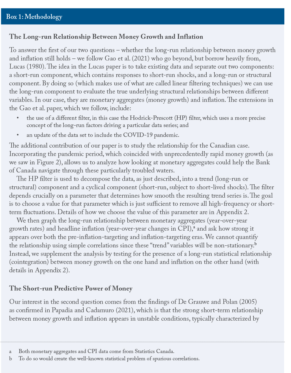
We discuss our methodology in detail in Box 1. We then present the main results along with our answers to the two questions above. The conclusion summarizes the results from the point of view of the Bank of Canada’s current conduct of monetary policy.

Results

We break down the results into the two questions.

Answer to Question #1

The first question is whether the long-run relationship between money growth and inflation still holds. To answer it we create the low-frequency or trend components for both money growth and inflation. Figure 3 shows how the trend component of our broad money measure (M2++) varies with trend inflation.

The results are striking. From the period from 1969Our data sample includes a little over a year of data from the fixed exchange rate period, which lasted until May 1970. This does not change the results. In fact, since it is generally recognized that monetary policy is less effective under fixed exchange rates, in principle, the results would be stronger if the sample was restricted to the flexible exchange rate period. to the late 1990s, the money growth and inflation paths are quite similar, with money growth clearly leading inflation. From about the turn of the century until the beginning of the pandemic, the trend inflation component remains very close to 2 percent (unsurprisingly, given the success of the Bank of Canada in hitting its target), while money growth is a little less stable, although not much.We perform the same exercise with M1++, M2+, and M3. The results are broadly consistent with this story, though the narrow M1++ measure is much more volatile in the post-2000 period.

The spike in M2++ at the end of the sample is due to the policy response of governments and the central bank to the pandemic. Households and firms received large transfer payments at the beginning of the pandemic, financed by borrowing. Household savings rates exceeded 25 percent in the second quarter of 2020, an unprecedented level.

Given the strength of the long-run relationship between money growth and inflation, we expect the recent uptick in inflation to be more than just a temporary phenomenon, with higher inflation for a period of time. The M2++ trend growth rate is approximately 1.5 percentage points higher than it was just before the pandemic in February 2020. Trend inflation has only recently started to catch up, and is now 0.7 percentage points above its pre-pandemic level.

For formal confirmation, we looked at evidence for cointegration – a meaningful long-run relationship that links particular variables – between money growth and inflation. As we discuss in Appendix 2, we find such a relationship both in the pre-inflation-targeting era, and, though more mixed, in the inflation-targeting era.The fact that it weakens in the back half of the inflation-targeting era is not surprising. We would argue that, on the whole, this dichotomy between the pre-inflation targeting and inflation targeting eras reinforces the point that the relationship between money growth and inflation becomes more apparent when inflation is unstable, as it is now. Using this relationship, we can test how quickly trend inflation will catch up to above trend money growth. Results suggest the catch up rate is approximately 4 percent per month, meaning – absent other economic shocks – the gap created by a change in trend money growth will be eliminated by higher trend inflation in a little over two years.

Answer to Question #2

Our answer to the first question makes clear that the long-run relationship between money growth and inflation holds. With money’s trend component increasing because of the pandemic, and with inflation yet to catch up, we expect the trend component of inflation to increase as well, keeping inflation elevated for a while yet

But this doesn’t tell us much about the short-run relationship: Can changes in money growth’s cyclical components tell us anything about the cyclical changes in inflation? Can we forecast inflation better using models that incorporate money growth?

Over the inflation-targeting era the answer has been no. That is not surprising since the best predictor of future inflation in a well-anchored inflation-targeting regime will be the target itself (see Otto and Voss 2014). However, with inflation spiking across the globe, and in Canada, where the most recent reading in May was 7.7 percent, there is a danger inflation expectations will become unanchored. Such a scenario might then mirror what we saw in the 1970s, when short-term money growth was a strong predictor of short-term inflation.

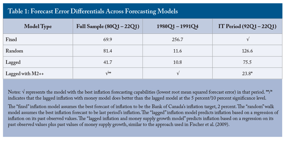
As mentioned above, we can test this theory using the empirical methodology found in Papadia and Cadamuro (2021). Specifically, using historical data, we can test different forecasting models, with one in particular containing information provided by monetary aggregates, and compare their forecast errors, where the lowest error rate shows the model with the best predictive abilities. We focus on broad monetary aggregates, and, in particular, M2++, given it had the tightest link to inflation in a structural sense (as we saw in Figure 3). Technical details concerning the regressions are in Appendix 2. The results are presented in Table 1.

In each column, the numbers indicate the increase in the root mean squared forecast error of a particular model, measured in basis points, compared to the best model over the given sample, which is indicated with a “√”.

The “fixed” inflation model assumes the best forecast of inflation to be the Bank of Canada’s inflation target, 2 percent. The “random” walk model assumes the best inflation forecast to be last period’s inflation. The “lagged” inflation model predicts inflation based on a regression of inflation on its past observed values. The “lagged inflation and money supply growth model” predicts inflation based on a regression on its past observed values plus past values of money supply growth, similar to the approach used in Fischer et al. (2009).

With respect to the inflation target being the best predictor of future inflation, it is not surprising that it does the worst of all in the pre-inflation-targeting period (column 2), and best of all in the inflation-targeting period (column 3). The random inflation model does poorly (relative to the others) in the inflation-targeting period and full sample, but does well in the pre-inflation targeting era.

Adding money to the lagged inflation model typically represents an improvement in forecasting ability. It does best overall in both the pre-inflation-targeting era, and the full sample model, the former consistent with the results of Papadia and Cadamuro (2021). Interestingly, as the ‘*’ signs indicate in the table, the difference between the lagged inflation and lagged inflation with money models is significant during the inflation-targeting (and full sample) period, but not in the pre-inflation-targeting period. That said, the coefficient (not shown) on money growth in the lagged inflation with money model is significant in the more unsettled pre-inflation-targeting era, and loses its significance if we restrict ourselves only to the inflation-targeting era.Results available upon request.

Combining our answers to the first and second questions, the implication of our results is that the loss of money as a significant predictor in forecasting future inflation lies not only in the Banks’ shift to inflation-targeting, but also in inflation being well anchored at the Bank’s target. In more unstable inflationary periods, such as the pre-inflation-targeting era and the current post-pandemic period, tracking money growth does indeed add value to forecasting models.

Policy Implications and Conclusions

Our results have strong policy implications. The Bank should monitor trend monetary growth more closely and track deviations of trend money growth from trend inflation, in particular when inflation is unsettled, as it is now. Such deviations are strong predictors of future changes in trend inflation. The results of our statistical tests show that if trend money growth changes – as it has to the tune of 1.5 percentage points higher than pre-pandemic – trend inflation catches up only gradually and with a lag. Trend inflation’s catch-up is only 0.7 percentage points so far, indicating more is to come Four percent of the gap created by a change in trend money growth is eliminated each month, so trend inflation, in the absence of other economic shocks, would catch up in a little over two years.

Our results have important implications for the analysis of monetary policy and inflation during the current pandemic period. Canadian monetary aggregates grew in 2020 and 2021 at unprecedentedly high rates, inflation is now nearly 6 percentage points above target, and measures of inflation expectations show that inflation is not expected to return to target within the Bank of Canada’s usual planning horizon of six to eight quarters. Money growth rates have come down in recent months, but it will take some time for trend inflation to follow this decrease. As a result, the Bank will have to work extra diligently to anchor inflation expectations. Accelerating its pace of quantitative tightening (QT) and continued forceful communications around the hikes to come should be part of this effort.

Monetary aggregates are relevant for predicting future changes to inflation. Money should be reintegrated by the Bank of Canada into its forecasting and monetary policy processes: more timely measures of these aggregates would be a good start in this regard.

Appendix 1: The Quantity Theory, Monetary Neutrality and Velocity

The quantity theory of money states that money times the velocity of circulation (velocity for short) is equal to nominal income. Mathematically,

Mt Vt = Pt Yt,

where Mt is a monetary aggregate, Vt is velocity, Pt is the price level, and Yt is real income (real GDP). Pt Yt is nominal income.

The equation is just an identity since velocity is defined to be the ratio of nominal income over the money supply. The theory gains predictive power when supplemented with the hypothesis that velocity is relatively stable (or at least predictable), depending in a reliable way on a small number of variables such as the opportunity cost of holding money (the appropriate nominal interest rate).

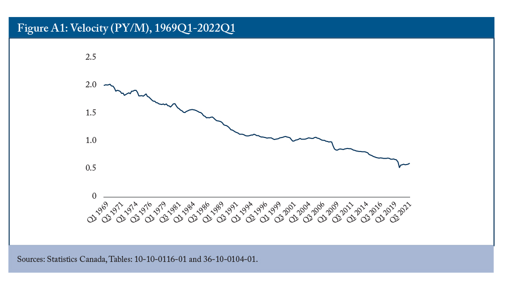
Velocity can fluctuate, especially in turbulent times. But, if it has a stable long-run average or follows a slow-moving trend (as it appears in Figure A1 using M2++ as our monetary aggregate), then an increase in money will be associated with a proportionate increase in nominal income. If money cannot affect real income in the long run (monetary neutrality), then an increase in money will lead to an increase in prices.Not quite proportionate since the change in real income (which is exogenous to money in the long run) has to be taken into account. See Friedman (2008) for more details on the quantity theory of money.

Appendix 2: Additional Methodology Notes and Results

Filtering the Data

For any time series yt (measured in logs, so that the first difference of the variable measures its growth rate), the Hodrick-Prescott filter calculates a long-term or trend component τt by solving the following constrained minimization problem:The cyclical component is just the original series minus its trend component, or (yt – τt).

The first term penalizes deviations of the original series yt from trend component τt. The second term penalizes abrupt changes in the growth rate of the trend component. The λ parameter governs how heavy the penalty is. When λ = 0, there is no penalty and the solution is to set the trend component equal to the series itself. As λ approaches infinity, the trend approaches a linear trend line.

Like Gao et al. we discipline the choice of λ to the appropriate business cycle narratives in Canada over our time frame. We test different values of λ to make this point clearer to the reader.

In order to extract out the appropriate low frequency data, we must ensure that the resulting series does not contain obvious cyclical features. Furthermore, the cyclical component must be consistent with a business cycle narrative that fits with real life results. We use the Bank of Canada’s Bank Rate,Data are more readily available on the Bank Rate than the Overnight Rate, which is actually the Bank of Canada’s monetary policy instrument. The two are very closely related. as in Gao et al., to help us create the cyclical narrative, as tightening cycles and loosening cycles tend to mimic the underlying business cycle.

It is helpful to think in terms of the Taylor rule (Taylor 1993), which fairly accurately models the behaviour of many central banks:

where it is the central bank’s policy rate, i* is the neutral rate of interest, πt is the inflation rate, π* is the inflation target, yt is real GDP, y* is potential GDP, and εt is an error term. The central bank aims to stabilize the economy around the inflation target and potential output. We want to choose λ such that (approximately) πt = π* and yt = y*, which removes the second and third terms, leaving only the influence of the slow-moving i* on the policy rate.

The default value of λ economists use to extract the long-run or low frequency component of a data
series follows Ravn and Uhlig (2002), who set  where pq is the number of periods per
quarter. This implies that for monthly data, with 3 months in a quarter, λ = 1600 × 34 = 129,600.

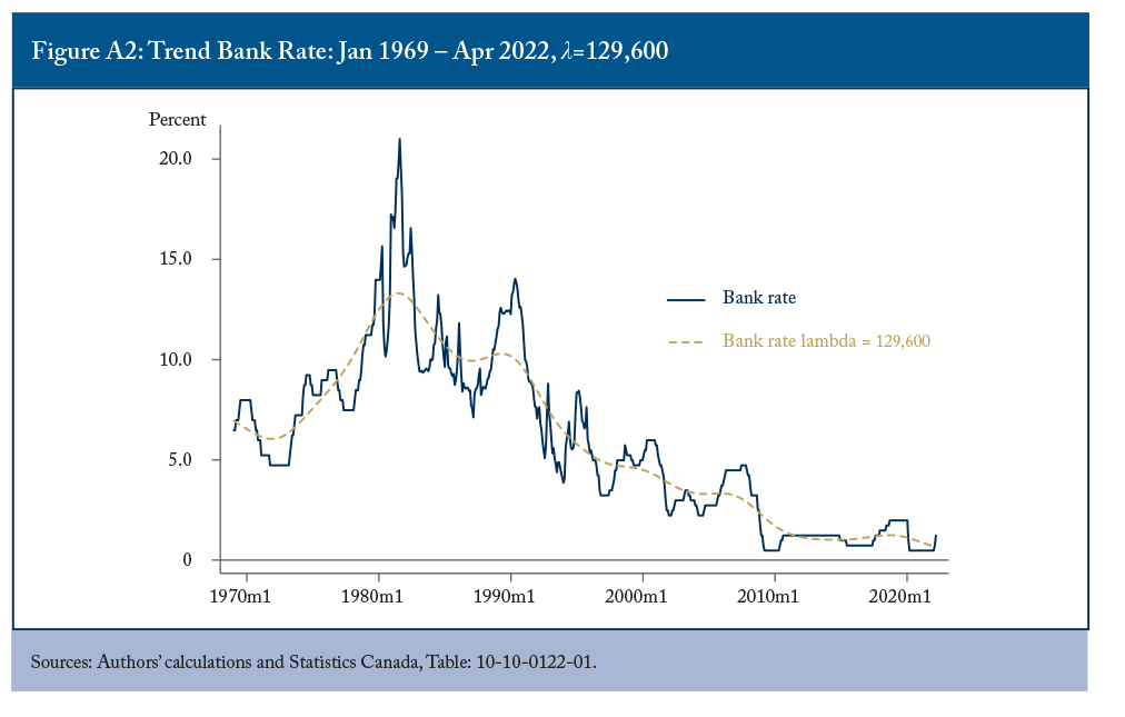
Figure A2 compares the actual Bank Rate with the low frequency Bank Rate using the Ravn and Uhlig smoothing parameter. The results indicate that this is likely too small a smoothing parameter since we can still quite clearly see when the Bank of Canada was undertaking particular tightening cycles.

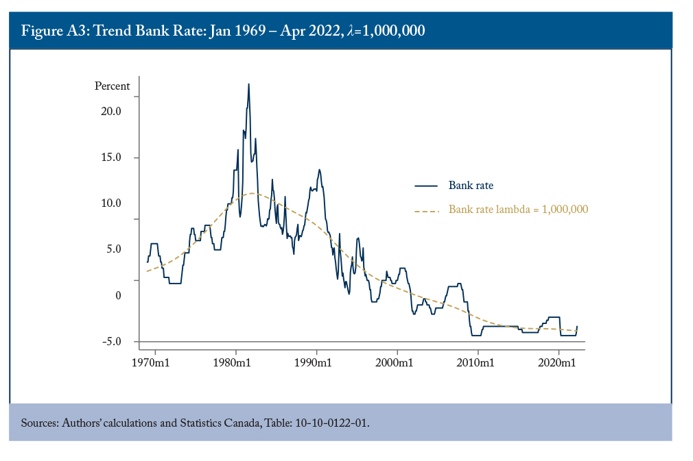
We then test an alternative, increasing λ to 1,000,000 (Figure A3). In this case, the low frequency data is much smoother and one cannot tell when the tightening cycles are occurring.

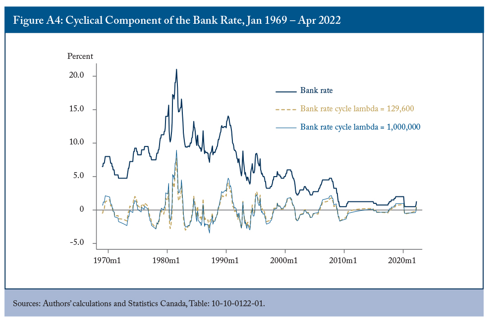
We must also ensure that the cyclical (high-frequency) data left over from the use of the larger λ is compatible with the actual Bank Rate. Figure A4 shows that this is the case. There is a clear improvement in the long-run trend component (since it eliminates visible cyclical components) without sacrificing the cyclical component.We note that the number of tightening cycles for each λ is 11, where we define the length of the cycles as the number of months in between two crossings of the zero horizontal line. We exclude any crossing that lasts less than 6 months. The average length of these cycles is 2-2.5 years, which is one year less than Gao et al. obtain for the US (3.5 years).

Cointegration Tests

Both of our variables of interest (money growth and inflation) have trends, meaning they are non-stationary variables. In such a context, correlation coefficients can be misleading: high correlations may be entirely spurious. Cointegration tests ask whether some linear combination of non-stationary variables is stationary.Technically, cointegration doesn’t have to mean non-stationary to stationary, it can simply mean going from an order of integration d to an order of integration less than d. If there is such a combination, the two variables are said to be cointegrated, and there is a meaningful long-run relationship that links the variables.

We looked at both the full sample period and inflation-targeting period to see whether there was a cointegrating relationship. Using a Johansen (1995) test for cointegration, we find that there exists such a long-run relationship between monetary aggregates and inflation, though with stronger results in the pre-inflation-targeting era, reinforcing the results we see in Figure 3 in the body of the text.Results available upon request.

When these cointegration relationships between variables exist, one can use what’s called an error correction model to determine the speed at which our dependent variable – in our case inflation – returns to its equilibrium after a change in the independent variable – in our case, money growth. We run a two-equation error correction model with the change in inflation and the change in money growth as the dependent variables. The equation for the change in inflation can be written as follows:

where π is the inflation rate, m is money growth, ∆ means a variable is differenced, and δi, α, and βi are coefficients. The term in brackets gives the cointegrating vector (i.e. the stationary linear combination of nonstationary variables) and α gives the speed of adjustment towards equilibrium if the vector is away from its equilibrium value.

We find βi to be equal to -0.818, which means there is close to a complete pass-through in the long term from money growth to inflation in our sample. While the absolute value of this coefficient gets much smaller in the inflation-targeting era, we argue that the environment we are currently in at least resembles some of the pre-inflation-targeting era, making the full sample calculation appropriate. Our estimate of the speed of adjustment coefficient α is -0.042. Both coefficients are significant at the 1 percent level. This means that if money growth is above its equilibrium value, inflation will catch up or converge to the different rate of money growth at the rate of 4.2 percent per month.

Short-term Prediction Models

The detailed specifications of the four different prediction models analyzed by Papadia and Cadamuro (2021) are as follows. The forecast errors of each model are used to calculate their mean squared forecast errors.

1.  Constant inflation: assume the best forecast of inflation is the Bank of Canada’s inflation target, 2 percent. In mathematical terms, πt = π* + εt, where πt is the predicted inflation rate at time t, π* is the inflation target, and εt is the forecast error.
2. Random walk inflation model: the best inflation forecast is last period’s inflation. In mathematical terms, πt = πt–1 + εt, where πt-1 is the previous period’s inflation rate.
3. The lagged inflation model: inflation is predicted based on inflation from the previous p periods, with weights based on the following regression: πt = a + b1 πt–1 + b2 πt–2 + ... + bp πt–p + εt, where the bi, i = 1 ... p are the estimated weights, a is a constant term, and where the choice of the number of lags p is based on the Akaike Information Criterion (AIC). Technically, this is what is known as an AR(p) model, where “AR” denotes “autoregressive.”
4. Lagged inflation and money supply growth model (or AR(p) with money): inflation is predicted based on both inflation and money supply growth from the previous p periods, with weights based on the following regression: πt = a + b1 πt–1 + b2 πt–2 + ... + bp πt–p + c1 xt–1 + c2 xt–2 + ... + cp xt–p + εt, where the bi, ci, i = 1 … p are the estimated weights, a is a constant term, and xt is money supply growth at time t. For consistency, we use the lag structure from model 3.

The full sample forecasting period extends from January 1980 to April 2022 at a quarterly frequency. The pre-inflation-targeting forecasting period runs from January 1980 to December 1991.As with the long-run analysis, the results do not change if we restrict the sample to include only the flexible exchange rate period beginning in June 1970. The sample forecasting period for the inflation-targeting period itself runs from January 1992 to April 2022. For tests which involve running regressions to estimate parameters prior to forecasting (the AR(p) model and the AR(p) with money model), the original sample period runs from January 1969 to December 1979 for both the full sample period and the pre-inflation-targeting period, and from January 1969 to December 1991 for the inflation-targeting period. Observations before January 1980 (or before January 1992 for the inflation-targeting period) are required to estimate the model’s parameters in order to initiate our out-of-sample forecasts. The optimal number of lags for the AR(p) model was one according to the Akaike Information Criteria test. As noted in the text, the regressions were re-run in every new forecast quarter to incorporate new information.

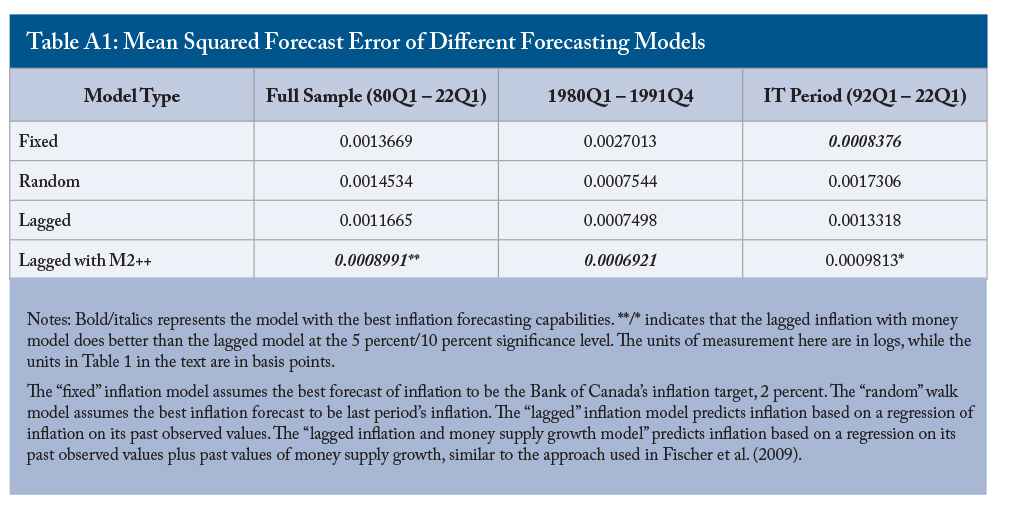
In the text we reported the root mean squared error differential across forecasting models. Here we report, as do Papadia and Cadamuro, the mean squared forecast error for completeness’ sake.

References

Ambler, Steve. 2022. “Quantitative Easing – Unintended Consequences.” Intelligence Memo. Toronto: C.D. Howe. May 25. Accessed at: https://www.cdhowe.org/intelligence-memos/steve-ambler-quantitative-easing-unintended-consequences

__________. 1989. “Does Money Matter in Canada?” Review of Economics and Statistics. 71: 651–658.

Bank of Canada. 2022. “Canadian Survey of Consumer Expectations—First Quarter of 2022.” Ottawa, Bank of Canada. Accessed at: https://www.bankofcanada.ca/2022/04/canadian-survey-of-consumer-expectations-first-quarter-of-2022/

__________. 2022a. “Business Outlook Survey—First Quarter of 2022.” Ottawa, Bank of Canada. Accessed at: https://www.bankofcanada.ca/2022/04/business-outlook-survey-first-quarter-of-2022/

Benati, Luca. 2009. “Long Run Evidence on Money and Inflation.” Working Paper 1027, European Central Bank. Accessed at: https://www.ecb.europa.eu/pub/pdf/scpwps/ecbwp1027.pdf

Benati, Luca, Robert E. Lucas Jr., Juan Pablo Nicolini, and Warren Weber. 2021. “International Evidence on Long-Run Mondey Demand.” Journal of Monetary Economics. 117: 43–63.

Bergevin, Philippe, and David Laidler. 2010. Putting Money Back into Monetary Policy: A Monetary Anchor for Price and Financial Stability. Commentary 312. Toronto: C.D. Howe. October.

De Grauwe, Paul, and Magdalena Polan. 2005. “Is Inflation Always and everywhere a Monetary Phenomenon?” Scandinavian Journal of Economics. 107: 239–259.

Fischer, Björn, Michele Lenza, Huw Pill, and Lucrezia Reichlin. 2009. “Monetary Analysis and Monetary Policy in the Euro Area 1999-2006.” Journal of International Money and Finance. 28: 1138–1164.

Friedman, Milton. 2008. “Quantity Theory of Money.” In: Palgrave Macmillan (eds.) The New Palgrave Dictionary of Economics. London: Palgrave Macmillan. Accessed at: https://doi.org/10.1057/978-1-349-95121-5_1640-2

Gao, Han, Mariano Kulish, and Juan Pablo Nicolini. 2021. “Two Illustrations of the Quantity Theory of Money Reloaded.” Staff Report 633, Federal Reserve Bank of Minneapolis. Accessed at: https://www.minneapolisfed.org/research/staff-reports/two-illustrations-of-the-quantity-theory-of-money-reloaded

Johansen, Soren. 1995. Likelihood-Based Inference in Cointegrated Vector Autoregressive Models. Oxford: Oxford University Press.

Laidler, David, and W. B. P. Robson. 1991. Money Talks – so Let’s Listen, Commentary 26. Toronto: C.D. Howe Institute.

Lucas, Robert E. Jr. 1980. “Two Illustrations of the Quantity Theory of Money.” American Economic Review. 70: 1005–1014.

Murray, Michael. 1994. “A Drunk and her Dog: An Illustration of Cointegration and Error Correction.” American Statistician. 48: 37–39.

Otto, Glenn, and Graham Voss. 2014. “Flexible Inflation Forecast Targeting: Evidence from Canada.” Canadian Journal of Economics. 47: 398–421.

Papadia, Francesco, and Leonardo Cadamuro. 2021. “Does Money Growth Tell Us Anything About Inflation?” Working paper 11/2021, Bruegel. Accessed at: https://www.bruegel.org/2021/11/does-money-growth-tell-us-anything-about-inflation/

Ravn, Morten O., and Harald Uhlig. 2002. “On Adjusting the Hodrick–Prescott Filter for the Frequency of Observations.” Review of Economics and Statistics. 84: 371–376.

Rowe, Nicholas, and James Yetman. 2002. “Identifying a policymaker’s target: an application to the Bank of Canada.” Canadian Journal of Economics. 35: 239–256.

Selgin, George. 2018. Floored! How a Misguided Fed Experiment Deepened and Prolonged the Great Recission. Washington DC: Cato Institute.

Serletis, Apostolos, and Zisimos Coustas. 2019. “Monetary Neutrality.” Macroeconomic Dynamics. 23: 2133–2149.