Calibrating Macroprudential Policies for the Canadian Mortgage Market

The Study In Brief

Macroprudential regulation has been on the rise since the 2007–09 global financial crisis. In Canada, the primary policy tools that have been employed in this regard are related to the residential housing market – namely, changes in mortgage loan-to-value ratios and loan maturity requirements. In this Commentary, we use an analytical model to forecast the probability of a state of low financial stability in the Canadian economy and recommend when policy action might be taken in light of its costs and benefits.

We project a low probability of low financial stability in Canada that rises gradually through year-end 2020, but remains low. This might seem odd given recent events around COVID-19. However, there are two things for readers to keep in mind. First, COVID-19 is a black swan event occurring in the real economy, one that does not originate in financial markets, making it difficult for financial regulators and policymakers to anticipate and model in advance. This is critical, as the goal of our paper is to provide a modeling tool to do just that. Second, once we have entered a downturn, financial regulators will not tighten a policy to head off financial instability. They will, in fact, do the opposite, by loosening policy rules to try and stimulate the economy.

Canada is an interesting case with respect to financial stability concerns and policies. Although the Canadian economy was able to stave off many of the negative effects of the last financial crisis, it continues to have growing levels of household debt. As a result, after loosening housing-related macroprudential policies in the lead-up to the crisis, policymakers have spent much of the past decade tightening these same policies.

Despite work analyzing the effects of housing-related macroprudential policies, there has been very little focus on advising policymakers about when to implement them. Any such advice naturally begins with identifying occasions when financial stability concerns are prominent and likely to remain so, which we refer to as “low financial stability states.” The model identifies three such episodes in Canada between 1990 and the middle of 2019: the early 1990s recession, the mid-1990s government budget rebalancing and the 2008 financial crisis. The four Financial Stability Indicators (FSIs) in our model specifications are the house-priceto-rent ratio, the price-to-income ratio, the debt-servicing ratio and the household-credit-to-GDP ratio. We then use the model to forecast the probability of entering another such episode over a two-year policy horizon. The model provides an answer to the question of whether the probability of entering and staying in a low financial stability state is high enough to go ahead with the policy, given the cost of implementation.

Our analysis suggests that, as of the second quarter of 2019, and abstracting from the black swan COVID-19 event, the probability of a lengthy period of low financial stability is low, extending to late 2020.

Introduction

Macroprudential policies, those with the aim of mitigating risk to the financial system as a whole, became more formalized and prominent after the 2007–09 global financial crisis as central bankers and financial regulators looked for tools to address future increases in systemic risk.

The design and implementation of these new policies have presented many challenges, not the least of which is determining when to enact them. In this Commentary, we first propose a set of financial stability indicators that could help Canadian policymakers forecast when financial stability is low and might require the use of these macroprudential policies. Second, and more important, we propose an analytical framework that maps these government forecasts into a decision-making process for implementing housing-related macroprudential policies, such as changes to required loan-to-value (LTV) ratios and maximum loan maturities for residential mortgages. Our focus on housing-related macroprudential policies reflects the importance of the housing market to the Canadian economy, in terms of both its contribution to gross domestic product (GDP) and the quantity of outstanding mortgage debt. The proposed framework should help policymakers decide when the benefits of a macroprudential (residential) mortgage policy might outweigh its costs.

Canada is an interesting case with respect to financial stability concerns and policies. Although the Canadian economy was able to stave off many of the negative effects of the 2007-2009 global financial crisis, it continues to have growing levels of household debt. As a result, after loosening housing-related macroprudential policies in the lead-up to the crisis, policymakers have spent much of the past decade tightening these same policies. In late 2006, loose policies reached their zenith, with maximum LTV ratios increasing from 95 percent to 100 percent, such that no downpayment was required to take out a residential mortgage loan. Similarly, over the course of 2006, the maximum loan amortization period gradually increased from 25 to 40 years. Once the crisis began, however – and given its genesis in the US housing market – these policies were mostly walked back. In October 2008, the LTV ratio was tightened to 95 percent and the maximum maturity reduced to 35 years. This tightening strategy has characterized much of the period since.

The effects of these policies before and after the crisis are well documented (see Allen et al. 2017; Kuncl 2016). However, despite work analyzing the effects of housing-related macroprudential policies, there has been very little focus on advising policymakers about when to implement them (see van Oordt 2018, for an example). Any such advice naturally begins with identifying occasions when financial stability concerns are prominent and likely to remain so, which we denote as “low financial stability states.” To identify these states, we use the modelling approach developed by Brave and Lopez (2019), which incorporates financial stability indicators. The model identifies three such episodes between 1990 and 2019 as periods of low financial stability within Canada: the early 1990s recession, the mid-1990s government budget rebalancing and the 2008 financial crisis. The model is then used to forecast the probability of entering another such episode over a two-year policy horizon. Again relying on Brave and Lopez (2019), we show how these forecast probabilities can be combined with calibrated policy costs and benefits to suggest if and when the policies should be implemented. The model provides an answer to the question of whether the probability of entering and staying in a low financial stability state is high enough to go ahead with the policy, given the cost of implementation. It does not, however, provide insight on the magnitude of the policy action. It is also agnostic with respect to monetary policy, in order to ensure macroprudential policy decisions occur in an environment where no assumptions are made about possible offsetting or amplification effects of other variables.

In the Canadian context, we project a relative low probability of entering a state of adverse financial stability as of mid-year 2019. This probability rises gradually through year-end 2020, but remains low. This might seem odd given recent events around COVID-19. However, there are two things for readers to keep in mind. First, COVID-19 is a black swan event occurring in the real economy, one that does not originate in financial markets, making it difficult for financial regulators and policymakers to anticipate and model in advance. This is critical, as the goal of our paper is to provide a modeling tool to do just that. Second, once we have entered a downturn, financial regulators will not tighten a policy to head off financial instability. They will, in fact, do the opposite, by loosening policy rules to try and stimulate the economy.

Returning to our findings, even in light of this low probability, it still might be prudent to enact macroprudential policies if the costs of a financial crisis were large enough. Based on our policycost calibrations, however, we would not advise policymakers to tighten housing policy rules in the near term, but things are less certain for later in the two-year horizon of our analysis.

Macroprudential Policies in the Canadian Context

Roles and Responsibilities

The first thing to understand about the Canadian financial system is the complex design of its regulatory system and the associated roles and responsibilities. As others have noted, the system is fragmented at both the geographic and functional levels (see, for example, Kronick 2018; Le Pan 2017). Deposit-taking institutions are fragmented between federally chartered banks – notably Canada’s Big Six – which come under the prudential supervision of the Office of the Superintendent of Financial Institutions (OSFI), and provincially regulated credit unions and caisses populaires, which are supervised by respective provincial regulatory commissions.¹1 Note that the Financial Consumer Agency of Canada regulates the market conduct of federally regulated deposit-taking institutions. Also, credit unions and caisses populaires, as of 2012, have had the option of voluntarily coming under the federal regulatory regime; for a variety of reasons, the uptake has been very slow. OSFI is also the federal prudential regulator of insurance companies – life and health, as well as property and casualty. The provinces, however, look after the licensing of insurers operating within their jurisdictions. Lastly, each province has its own provincial securities commission, although the Cooperative Capital Markets Regulatory System was created with the goal of bringing all these bodies under one roof. Notably, only about half the provinces and territories have joined, with the critical provinces of Quebec and Alberta abstaining.²2 Naglie (2017) provides a detailed discussion of the history of the search for a national securities regulator and why the Cooperative Capital Markets Regulatory System is unlikely to bring everyone under the same tent.

All this to say that Canada does not have a prudential regulator solely in charge of assessing financial systemic risk, which is at odds with the trend post-crisis, in which many countries have turned toward single or twin regulator models (see Edge and Liang 2019 for further discussion). Indeed, the International Monetary Fund (IMF) has criticized Canada for a lack of regulatory harmonization and the need to have a body in charge of systemwide financial risk (see IMF 2014a).³3 Although, to be fair, the IMF has also given Canada high marks for a regulatory framework that is “strong, and complemented by a credible federal system of safety nets” (IMF 2014a, 6), as well as noting that Canada’s “framework for the regulation and supervision of securities markets demonstrates a high level of implementation of the [International Organization of Securities Commissions] principles” (IMF 2014b, 5). Although Canada does have four different coordinating bodies that provide this oversight, no one body is charged with macroprudential supervision (for details, see Kronick 2018).⁴4 The four bodies are the Financial Institutions Supervisory Committee (FISC), the Senior Advisory Committee, the Heads of Agencies and the Canadian Securities Administrators Systemic Risk Committee. Only FISC is statutory. This highlights the need for carefully designed macroprudential policies, as well as research that contributes both to our understanding of financial system vulnerabilities and to our ability to determine when to implement a given policy.

The Housing Market

Given these complexities, we narrow our focus here on macroprudential policies related to the residential housing market – specifically, on changes to the maximum loan-to-value (LTV) ratio and amortization length undertaken between 1990 and 2015. We note that this period excludes recent changes by the federal government and OSFI to mortgage qualification rules,⁵5 Changes came in 2016 for high-ratio mortgages (mortgages with LTV ratios greater than 80 percent) and in 2018 for lowratio mortgages (those below 80 percent). which included an expanded stress test to determine whether borrowers could still afford their mortgage if interest rates were to rise. While quantifying the effects of these changes has begun (see, for example, Bilyk and Tenyenhuis 2018), it is too early to calibrate their full impact on the economy, which is necessary for the empirical work we perform.

We focus on the housing market for a variety of reasons, including its frequent identification as Canada’s most significant risk (notwithstanding the recent global pandemic, COVID-19). As the Bank of Canada notes in its May 2019 Financial System Review, [p.6] “[o]verall, the vulnerability associated with high household indebtedness remains significant, although it has declined modestly. As households adjust to changes in mortgage policies and past increases in interest rates, the pace of borrowing has slowed and the quality of new mortgages has improved. Nonetheless, a large amount of debt in Canada is held by highly indebted households.” In support of this view, IMF data suggest that Canada ranked seventh out of 79 countries in household debt as a percentage of GDP in 2017.⁶6 The top-ranked country would have the highest household debt as a percentage of GDP.

To gauge financial system vulnerabilities in Canada, Duprey and Roberts (2017) introduce a “vulnerabilities barometer.” Of the 28 variables making up this barometer, 17 incorporate housing to one extent or another and 10 focus directly on housing debt. Figure 1 shows the ratios of household mortgage debt to GDP and household mortgage debt to disposable income. The figure indicates the extent to which these two debt measures increased in Canada both pre- and postfinancial crisis, and show why policymakers have placed so much emphasis on household debt.

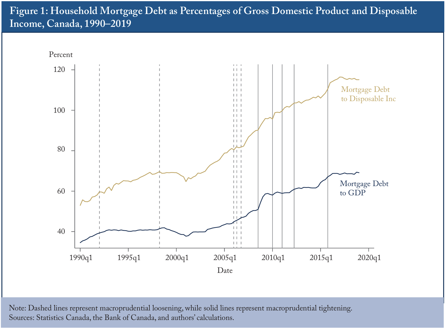
This concern has manifested itself since 2008 in a series of macroprudential tightenings in the government-backed mortgage insurance program (see Table 1).⁷7 Federally regulated lenders must obtain mortgage insurance for borrowers who put down less than 20 percent of the purchase price of the home. The cost of the insurance premium is passed down from lender to borrower. The government backs 100 percent of Canada Mortgage and Housing Corporation’s mortgage insurance obligations if it is unable to make payouts to lenders, and 90 percent of the obligations of the two private mortgage insurers. While the focus on insured mortgages excludes the uninsured portion of the mortgage market, presumably policy tightening related to housing is likely to have its greatest effect on those making smaller downpayments – that is, those requiring insurance. In any event, recent analysis suggests that these tightenings have been successful in slowing down growth in aggregate mortgage debt ratios – the solid lines in Figure 1 appear to support such a claim.

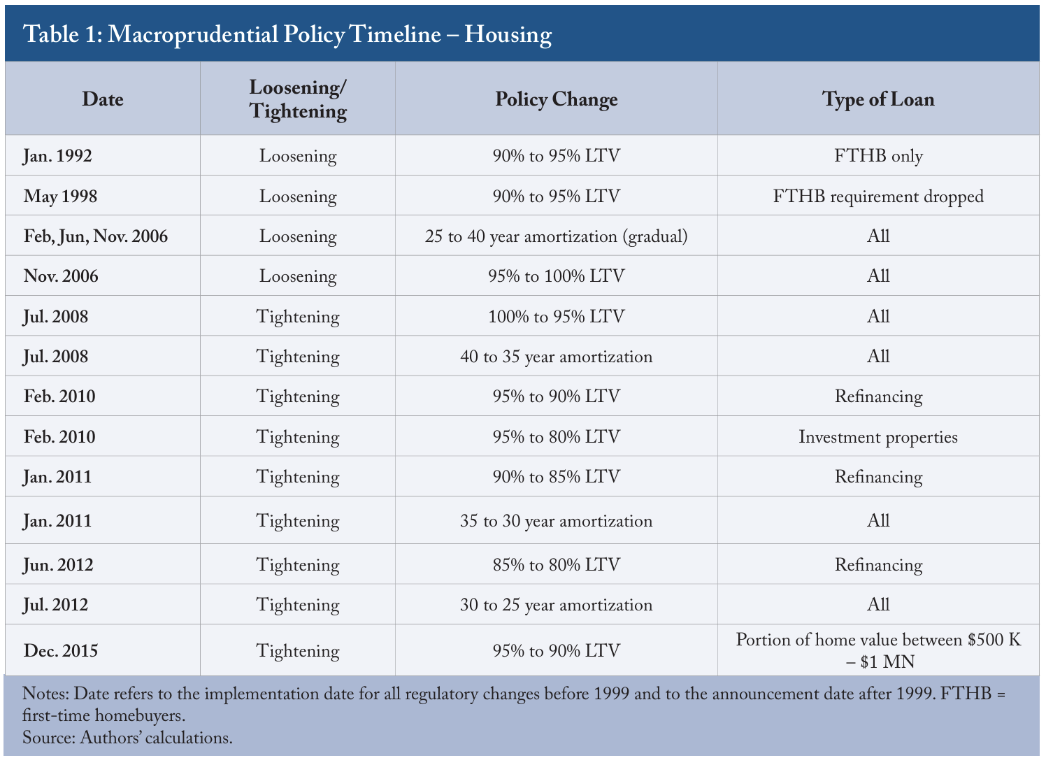
Others have found similar results. Kuncl (2016), studying the effect of macroprudential policy changes (related to insured mortgages) on residential mortgage credit and residential investment growth over the 2008–12 period, captures four rounds of regulatory tightening. The 2010 tightening of LTV ratios for refinancing and investment properties resulted in a 2.78 percentage point decline in mortgage credit.⁸8 The February 2010 tightening also required borrowers to be able to afford a mortgage at the five-year fixed rate even if they take out a mortgage at a lower interest rate and a shorter term. The other three periods of policy tightening – in 2008, 2011 and 2012 – mixed the tightening of both LTV ratios and amortization, resulting in a decline of 2.55 percentage points, an increase of 2.23 percentage points and a decline of 2.36 percentage points, respectively. As Kuncl (2016) points out, the increase in 2011 was likely due to the anticipation of a future tightening that led to a temporary rise in the demand for mortgage credit.

Allen et al. (2017) study changes in macroprudential insured mortgage policy using both loan-level and household survey data over the 2005–10 period for first-time homebuyers, who arguably are most affected by such policy changes in the near term. They find, for example, that the June 2008 tightening of the LTV ratio from 100 percent to 95 percent resulted in a 51 percent decline in loan qualifications, a 7.9 percent decline in firsttime homebuyers and an 8.1 percent decline in mortgage credit over a one-year period. Similarly, although with smaller magnitudes, the January 2011 tightening of the maximum amortization period from 35 to 30 years led to a 4.8 percent decline in loan qualifications, a 3.6 percent decline in first-time homebuyers and a 7.2 percent decline in mortgage credit. Tightening the LTV ratio has a greater effect because, although interest rates have been low since the financial crisis, asset values have increased, making the downpayment requirement more restrictive for first-time homebuyers, who typically have not built up a large wealth base.

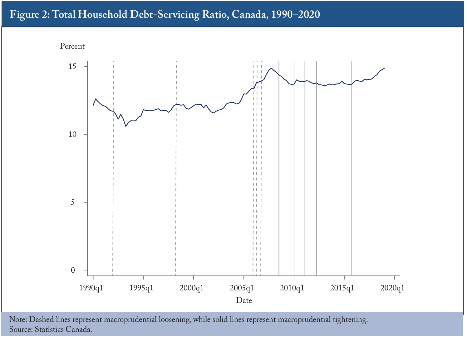
In many ways, falling interest rates and increasing asset values have offset each other when it comes to how much debt households must repay each month as a percentage of their disposable income – commonly referred to as a household’s debt-servicing ratio (see Figure 2 and Kronick 2017 for more detail). Higher housing prices have also resulted, however, in larger required downpayments. The implication is that households are likely more sensitive to any policy changes that affect wealth, such as changes to LTV ratios, but have more flexibility when it comes to policies that affect debt servicing, such as a change to amortization, which, when tightened, increases the amount households have to pay each month.

Despite Canada repeatedly being flagged for its rising household debt, there has not been a significant housing market correction over the past decade.⁹9 According to OECD data on housing prices, in the 40 quarters between 2009:Q3 (the first quarter after the recession) and 2019:Q2, the real housing price index has grown at a negative clip only seven times. Of these seven, the index dropped by more than one point only twice. https://data.oecd.org/price/housing-prices.htm. There are no doubt many reasons for the robustness of Canada’s housing market during this period, such as population growth and low unemployment, but another potential explanation is a flat debt-servicing ratio. The only period when debt-servicing ratios increased notably over the past 25 years was during the lead-up to the financial crisis, although there are some recent indications that they are on the rise again.

The cause of the increase in the debt-servicing ratio before the financial crisis was likely the loosening of the LTV ratio from 95 percent to 100 percent in November 2006. Not surprisingly, Allen et al. (2017) find much larger changes in loan qualifications, first-time homebuyers and mortgage credit from this loosening. The authors argue that these numbers are an overestimation related to the disappearance of any form of wealth constraint when a downpayment is not required. While true, the fact that this particular loosening has a more significant effect is, in our view, not surprising. Further, the finding highlights that it is not necessarily increases in credit that lead to corrections or financial crises, but the extent to which these increases cause debt-servicing ratios to rise. This view is consistent with the work of Kronick and Ambler (2020) for Canada and Drehmann, Juselius, and Korinek (2017), who, in a panel analysis that includes Canada, find that “debt service is the main channel through which new borrowing affects the probability of financial crises” (p.3). Therefore, if debt-servicing ratios have remained flat, despite an environment in which interest rates have long been low and household debt has been rising, perhaps it is not surprising that Canada has avoided the type of dire scenario oft-predicted for the housing market. However, the recent rise in household debt-servicing ratios and their importance to our model, to which we turn next, provide further impetus to study the macroprudential decision-making process.

A Framework for Analyzing Macroprudential Policies

As noted above, macroprudential policy is a relatively new responsibility for policymakers, and certainly less familiar and examined than monetary policy. Accordingly, an important first step in analyzing macroprudential policy is to develop an objective function – that is, an explicit, even if simplified, statement of the relative costs and benefits of a policy action. In general, deriving an objective function for this purpose requires detailed knowledge of the underlying decision problem. Although such knowledge is often not readily available due to limited historical experience, our focus on the Canadian housing market allows us to leverage recent studies, including the work of Kuncl (2016) and Allen et al. (2017), described above.¹⁰10 We do not consider the effects of these macroprudential policies at the provincial or subnational level since publicly available data are insufficient at these levels. This is an interesting line of future research – and an important consideration for policymakers.

We follow the approach developed by Brave and Lopez (2019), who specify a loss function based on deciding whether to enact or delay a costly policy action that could prevent financial instability. This allows a regulator to have an idea ex ante of what types of losses are expected if financial instability arises, which is in part determined by the timing of implementing a policy that itself has costs.

As developed by Kahn and Stinchcombe (2015), the analytical framework is applied at a point when a policymaker must decide whether to enact a costly policy to forestall the arrival of an adverse event, either immediately or in the near future. The intuition is that the policymaker faces uncertainty as to when the adverse event might arrive, and must decide whether and when to act preemptively. If the optimal policy action derived from the framework suggests that a policy should be delayed for a particular period of time, the situation can be monitored and optimal timing reevaluated as more information becomes available.

A key element of the Kahn and Stinchcombe framework is a hazard function of the arrival of such an adverse event. That is, the policymaker needs to generate a probability forecast of the adverse event arriving over a specified period. This probabilistic assessment is combined with the relative costs of enacting a particular policy, and used to solve for the optimal policy implementation date.

The optimal decision about when to act should balance the expected benefits of waiting (that is, inaction) with the expected costs of the event arriving after the policy has been implemented. Below, we discuss how this simple framework can be used to analyze when to implement macroprudential (residential) mortgage policies.

The Adverse Event and Its Probability

Applying the Kahn and Stinchcombe (2015) framework to Canadian housing policy requires that we specify the adverse event that would justify its implementation. The one we consider is an extended period of housing market instability – including, potentially, a financial crisis. We do not rely on a single financial stability indicator, but instead weight five indicators based on our empirical analysis. To generate the needed hazard function for this adverse event, we propose a Markov-switching model (as per Brave and Lopez 2019) that incorporates the information in financial stability indicators (FSIs) that are focused on the mortgage market. Our chosen list of FSIs is far from exhaustive, but as we discuss below, they capture episodes of stress in Canadian residential mortgage markets well. We note that, while the COVID-19 story is obviously a significant stress on economies all over the world, including Canada’s, its impact on the housing market at present is too soon to gauge, and this type of black swan event is nearly impossible to predict for regulators and policymakers looking at financial stability indicators.

In our baseline model, we focus on the interplay between growth in real household spending, new borrowing and the unemployment rate, where we define household spending as the sum of personal consumption expenditures and residential investment.¹¹11 To deflate both spending and borrowing, we use the Canadian consumer price index (CPI). Next – and given our discussion earlier on Canada’s avoiding a large housing market correction despite a rising ratio of household debt to GDP – we extend the model by incorporating additional FSIs that encompass different elements of the household side of the macroeconomy. In particular, we include the ratios of house prices to rent and house prices to income that Duprey and Roberts (2017) found to be useful “earlywarning” indicators of adverse developments in Canadian mortgage markets. We also include the debt-servicing ratio highlighted by Kronick (2017) and Kronick and Ambler (2020).¹²12 The source of our household credit data is the Bank of Canada, and includes both residential mortgage credit and consumer credit, excluding mortgages. The remaining FSIs are from Statistics Canada. We obtained most measures, however, from various Haver Analytics databases. We also test the traditional ratio of household credit to GDP (as in Duprey and Roberts 2017) as an additional FSI. Rather than rely on a single FSI to guide policy decisions, we instead weight each of our five model-implied hazard functions – one each for our baseline specification and four FSI specifications – according to its historical ability to signal instability in Canadian mortgage markets.¹³13 We follow the empirical Bayesian model averaging method proposed in Brave and Lopez (2019). Note that the four FSIs in our model specifications are the house-price-to-rent ratio, the price-to-income ratio, the debt-servicing ratio and the household-credit-to-GDP ratio. The fifth model specification is the baseline model, which does not include an FSI. An advantage of this simple procedure is that it readily allows for our analysis to be extended by others to include additional FSIs that might become necessary with the passage of time.

The Costs and Benefits of (In)Action

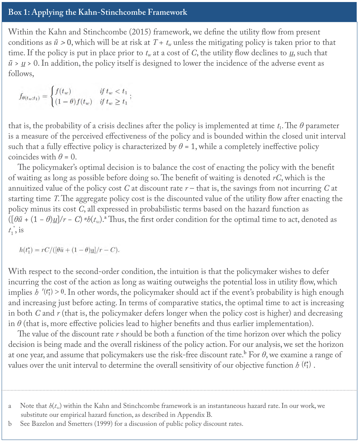
Translating macroprudential residential mortgage policy into the Kahn and Stinchcombe (2015) framework requires the calibration of the costs and benefits of such a policy action. Of course, there are many ways to measure benefits and costs, and ours is but one. A more formal, theoretical discussion can be found in Box 1, but the key point is that, within the Kahn and Stinchcombe framework, some kind of utility is at risk in the near future unless a mitigating policy is taken in advance. The policy has a cost, however, if enacting it causes the utility flow to decline, although by less than if the policy had not been implemented and the crisis had occurred. The magnitude of this utility cost, where the policy is implemented and the crisis avoided, is less severe the closer to the period of instability. Therefore, the policymaker’s optimal decision is to balance the cost of enacting the policy with the benefit of waiting as long as possible before doing so. Moreover, the policymaker should act if the event’s probability is high enough and is forecast to become more likely. Notably, these are characteristics of the empirical hazard functions for periods of low financial stability in Canada that we find in our empirical analysis.

Our approach to operationalizing the Kahn and Stinchcombe framework is to calibrate it to the costs and benefits of enacting macroprudential (residential) mortgage policy – in particular, the adjustments to LTV ratios in the governmentbacked mortgage insurance program. We use the work of Kuncl (2016) and Allen et al. (2017) as a guide. In both cases, we calibrate the policy costs in terms of lost economic activity due to the tightenings of housing market policy listed in Table 1. The input parameters for our policy calibrations are listed in Table 2.¹⁴14 Note that reduced mortgage access affects not only present-day consumption of housing services, but also the ability of households to smooth consumption over time. It is difficult, however, to make assumptions regarding consumption smoothing, so we take the difference between the expected one-year mortgage issuance growth rate and the policy-adjusted issuance growth rate calibrated using the Kuncl (2016) results as a proxy for the more complete picture of reduced mortgage access. Moreover, from the policymaker’s perspective, what is critical when deciding on the need to tighten macroprudential policy is the short-run horizon.

As discussed, Kuncl (2016) examines the decline in economic activity after these policy tightenings from 2008 to 2012 – that is, rows five through twelve in Table 1. We consider this reduced activity as our baseline measure of the cost of enacting these macroprudential policies. In particular, we focus on policy tightening regarding the LTV ratio for different categories of insured mortgages.

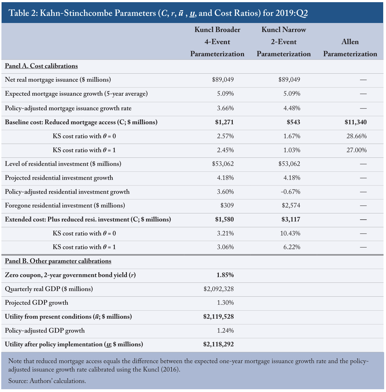
The first policy cost we consider is lost access to credit by mortgage borrowers, measured as the observed decline in residential mortgage credit growth. This measure is calculated as the difference between the “policy-adjusted mortgage issuance growth rate” and the “expected one-year mortgage issuance growth rate” shown in Table 2. We perform this calibration using all four policy events between 2008 and 2012 (column 1) and the latter two events in 2011 and 2012 (column 2).

As an example, new mortgage origination in real terms by mid-year 2019, according to Statistics Canada, was $89.0 billion. Average growth in mortgage credit over the previous five years was 5.09 percent. If we use Kuncl’s (2016) reported average expected growth in mortgage credit with and without the implementation of a particular macroprudential policy, we get a difference of 1.43 percentage points, dropping the 5.09 percent average mortgage credit growth to 3.66 percent. A decline of 1.43 percentage points means a loss of residential mortgage credit of $1.3 billion (1.43 percent of $89.0 billion). We denote this as the baseline cost in the Kuncl 4-event column.

We then consider an extension of our cost calibration. Namely, we add to the lost residential mortgage credit growth the decline in average residential investment growth after these tightening policies were enacted. This measure is calculated as the difference between the “policy-adjusted residential investment growth rate” and the “projected residential investment growth rate” in Table 2. Admittedly, monetary policy might intervene if residential investment growth were to fall, but there are at least two reasons for policymakers to consider this extended cost for macroprudential purposes only. First, it is important for them to understand the environment, assuming other variables are fixed. Second, in Canada, decisions related to macroprudential policy in the housing market and monetary policy are performed by separate institutions (the federal Department of Finance and OSFI for the former and the Bank of Canada for the latter).

Again, using the same Kuncl 4-event column example, we take the level of real residential investment at mid-year 2019 ($53.0 billion), and calculate the average one-year growth rate over the previous five years (4.18 percent). We again use Kuncl’s average expected one-year growth in residential investment with and without macroprudential regulation implementation to determine the expected loss in this variable, a decline from 4.61 percent to 4.03 percent, or 0.58 of a percentage point. This decline costs $309 million in forgone residential investment growth, raising the overall cost to $1.6 billion ($1.3 billion + $309 million).

For the alternative policy costs implied by Allen et al. (2017), we focus on first-time homebuyers and, in particular, on the decline of about 8 percent in the number of first-time homebuyers after the policy tightening in 2008. We estimate that, as of year-end 2016 (the most recent available data), mortgages for such buyers totalled about $140 billion, based on roughly 480,000 mortgages with an average balance of $290,675, according to data from Canada Mortgage and Housing Corporation. Accordingly, the decline in first-time homebuyers’ access to credit would be about $11.3 billion, as shown in the third column in Table 2.

The bottom panel of Table 2 presents our calibrated values for the other input variables from Kahn and Stinchcombe (2015). The lower and upper utility flows are challenging to define accurately, especially for occasions when there is limited historical experience with a policy action. Accordingly, we consider the growth of real GDP as the most likely measure of policymakers’ concerns and utility flows. We use real GDP in Canadian dollars for the year in question to set the analytical starting point, and the forecasted one-year GDP growth rate from the Bank of Canada’s Monetary Policy Report to set the expected real GDP level at the end of the following year. This dollar measure represents the expected utility flow over the year, and is a measure of utility in the case where there is no crisis event and the policy was not implemented (that is, the upper utility flow). The corresponding calculation of no crisis event with policy implementation requires a downward adjustment to the forecasted real GDP growth rate as calibrated to the policy action in question (that is, the lower utility flow). For our adjustment, we use the average decline of 0.58 of a percentage point in residential investment growth after policy implementation, as reported by Kuncl (2016). This reflects the difference between “policy-adjusted residential investment growth rate” and “projected residential investment growth rate” in Table 2, column 1. Accordingly, since residential investment is about 10 percent of total GDP, we scale the policyadjusted GDP growth rate to a decline of about 0.058 of a percentage point.¹⁵15 Box 1 has further detail on the required calibration of both the discount rate and the perceived effectiveness of the policy in lowering the likelihood of the adverse event.

Transforming Financial Stability Indicators into Hazard Functions

In this section, we describe the mechanics of our estimation procedure and how to translate our probabilities of Canadian mortgage market instability into the hazard functions necessary for the Kahn and Stinchcombe (2015) framework.¹⁶16 Appendix A has further details on our Markov-switching models, as per Hamilton (1989).

The Model

Our model is meant to capture the joint dynamics of growth in real household spending and borrowing in order to identify distinct states of high and low stability for the Canadian mortgage market. That is, we model the transitions between these two states based on changes in the correlation between real household spending growth, its onequarter-lagged value, and one-quarter-lagged values of real growth in household borrowing and changes in the unemployment rate. The model is estimated over the period from the first quarter of 1990 through the second quarter of 2019.

We introduce our four FSIs into the model, on an individual basis in order to limit the number of estimated parameters. Correspondingly, our approach uses five model specifications, as discussed earlier. To arrive at a single characterization of the state of mortgage market stability, we weight each model by a measure of its fit to the data, giving more weight in relative terms to models that best capture the estimated transitions in the Canadian data (see Appendix B for further details).

States of Financial Stability

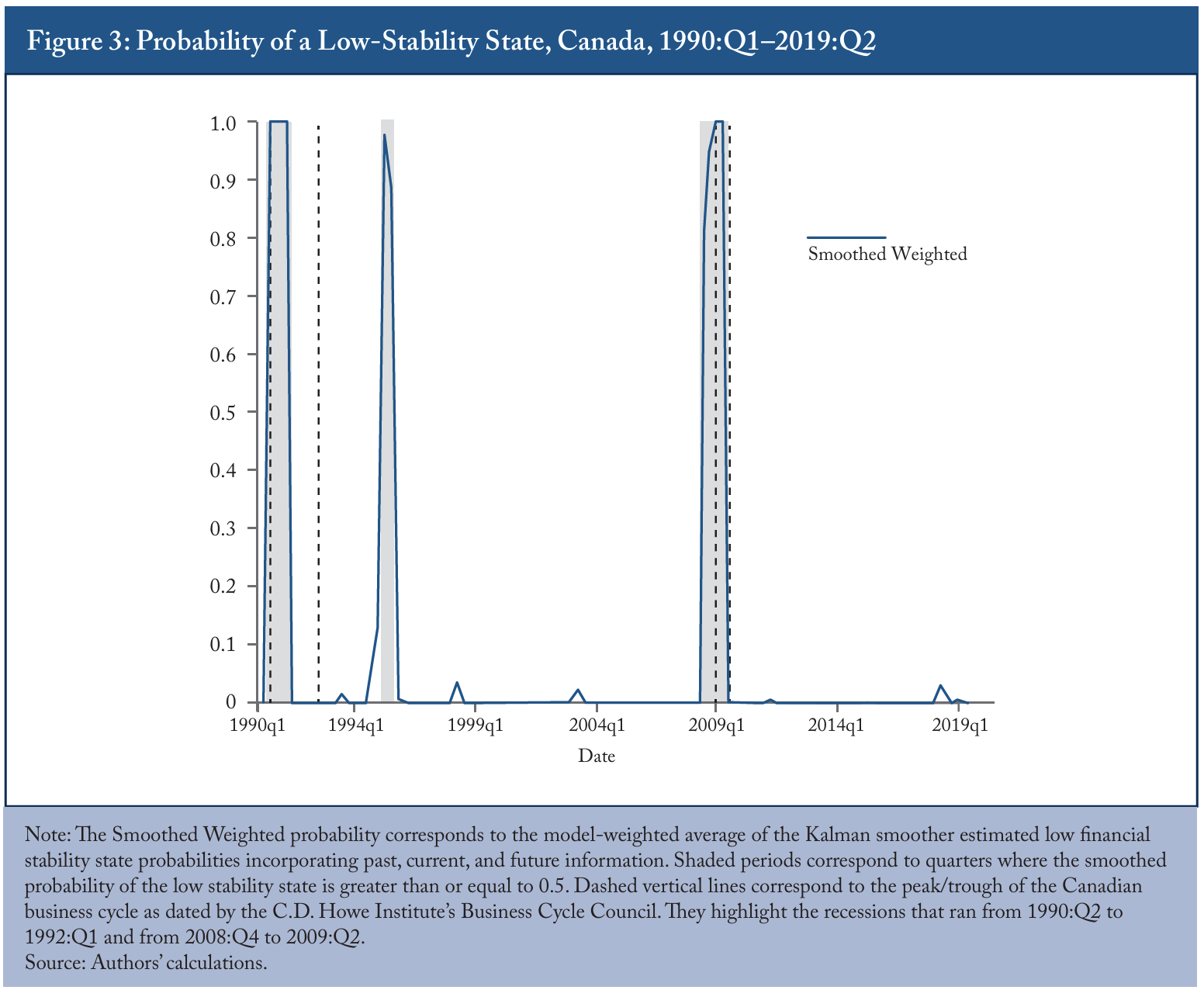
Figure 3 shows estimates of the model-implied probability of the low-stability state for mortgage markets, weighted across our five specifications. The shaded regions in the figure denote quarters where the probability of the low-stability state exceeds 50 percent, while the dashed (black) lines mark the peaks and subsequent troughs of the Canadian business cycle (as dated by the C.D. Howe Institute’s Business Cycle Council). The three, model-implied periods of low stability are 1990:Q2 to 1991:Q2, 1995:Q1 to 1995:Q2 and 2008:Q3 to 2009:Q1. Each corresponds to well-known periods of stress: the early 1990s recession, the longest in Canada since the Great Depression; the mid-1990s rebalancing of the federal budget from a deficit of 6 percent of GDP in 1995 to a balanced position two years later; and the 2008–09 global financial crisis. Although other minor periods of stress in 1998, 2003 and early 2018 are suggested by the model, its overall fit to the data and actual events in the macroeconomy suggests its usefulness for our analysis.

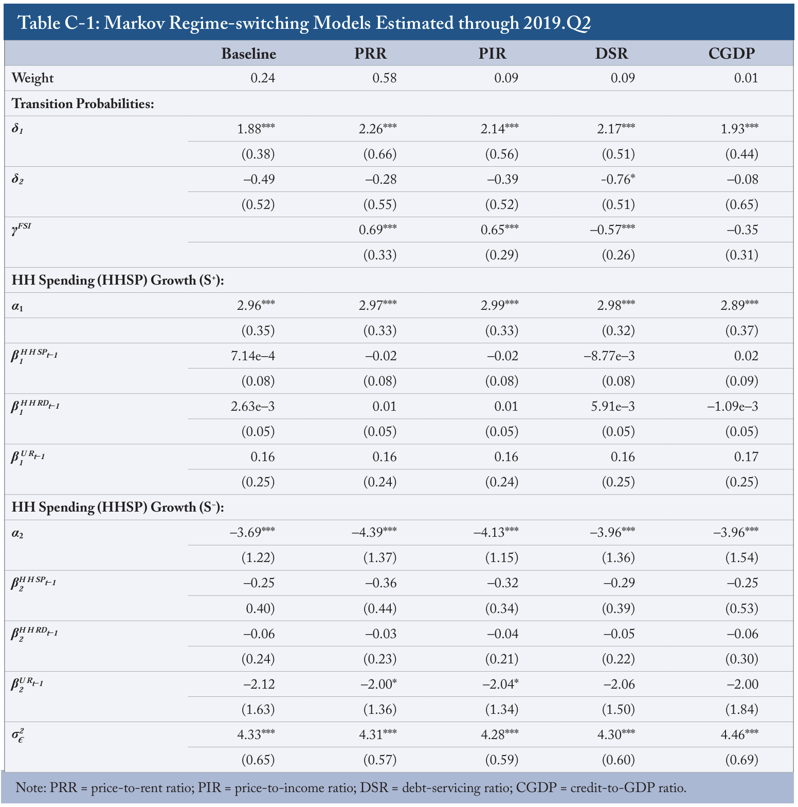
To examine our results more rigorously, Table C-1 in Appendix C presents the estimated coefficients for our five model specifications – that is, our baseline model without any FSI and that model augmented with a single FSI, whether the price-to-rent ratio, price-to-income ratio, debtservicing ratio or credit-to-GDP ratio. Starting with our baseline specification, it is clear that transitions from one state of financial stability to another are largely characterized by differences in average real spending growth – that is, it is positive in the high-stability state and negative in the low-stability state. Lagged spending and debt growth and changes in the unemployment rate, on the other hand, are not significant predictors. This situation changes, however, when we add several of the FSIs to the model. In particular, increases in the unemployment rate predict large declines in household spending in the low-stability state.

Appendix Table C-1 also shows that, with the exception of the household-credit-to-GDP ratio, the introduction of the other FSIs (γFSI) tends to have significant direct effects on the probability of transitioning from one stability state to another. The insignificance of the credit-to-GDP ratio is contrary to its importance in Duprey and Roberts (2017), but is consistent with the idea that, as interest rates have fallen, house prices have increased. The result is that the credit-to-GDP ratio has increased without changing the amount households must pay out of disposable income in a given month – that is, the debt-servicing ratio has remained flat. The most significant cases, on the other hand, are for the price-to-rent and priceto-income ratios, consistent with the importance of these variables in Duprey and Roberts’s vulnerabilities barometer. However, the positive coefficients suggest that, as these ratios rise over time, the probability of transitioning to the lowstability state in the next period decreases, making these variables poor leading financial stability indicators. In contrast, the debt-servicing ratio has a negative coefficient, suggesting that, as this ratio rises over time, the probability of transitioning to the low-stability state increases. In other words, the debt-servicing ratio acts as a leading indicator of financial vulnerability, consistent with the work of Drehmann, Juselius, and Korinek (2017) and Kronick and Ambler (2020).¹⁷17 Note that the 0.09 does not imply that the debt-servicing ratio provides little value added. Because much of the information on debt servicing is caught up in the model’s credit variable, debt servicing must work that much harder to provide additional information. What is critical is that it is the only financial stability indicator to act as a leading indicator.

Forecasts of Financial Stability

To use these model-implied probabilities of financial stability in our policy assessment framework, we need to project them out over the time horizon of interest. This procedure allows us to generate forecast probabilities over the number of quarters in the policymaker’s decision horizon.

We follow Brave and Lopez (2019), who assume that policymakers are concerned with the probability of four consecutive quarters of financial instability, and project our hazard function at time T for this event over an eight-quarter horizon. This is consistent with Drehmann and Juselius (2013), who argue that FSI signals should have appropriate timing to be useful for macroprudential policy responses, with signals arriving at least six quarters before a potential crisis. The early warning indicator nature of several of our FSIs, therefore, should be useful for guiding macroprudential (residential) mortgage policy decisions over this time horizon.

Transforming Hazard Functions into Policy Recommendations

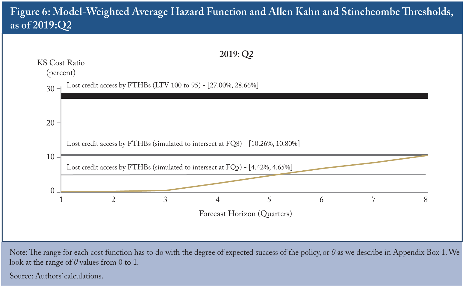
Based on the calibrated costs and benefits of enacting this macroprudential mortgage policy and our projected hazard function of being in the low financial stability state for four quarters, we can turn to the question of relevance for policymakers: forecasting whether it would be advisable to enact macroprudential residential mortgage policies in the period after our data ends. In particular, with 2019:Q2 as our starting point, we examine two sets of policy actions. The first one is the policy tightenings examined by Kuncl (2016), including both the average effect across all four policy tightenings between 2008 and 2012 (Figure 4) as well as the average of just the latter two events (Figure 5). The second set of policy actions we examine are the policy tightenings from Allen et al. (2017), that focus more directly on first-time homebuyers (Figure 6).

In Figure 4, the baseline cost we consider – that is, just the decline in residential mortgage credit growth – is shown on the left. The extended cost graph on the right depicts the decline in that growth plus the decline in residential investment growth. In both panels of Figure 4, the projected hazard functions (the upward-sloping line) for four consecutive quarters of low financial stability are the same; the only difference is the policy cost calibrations (the shaded lines). 

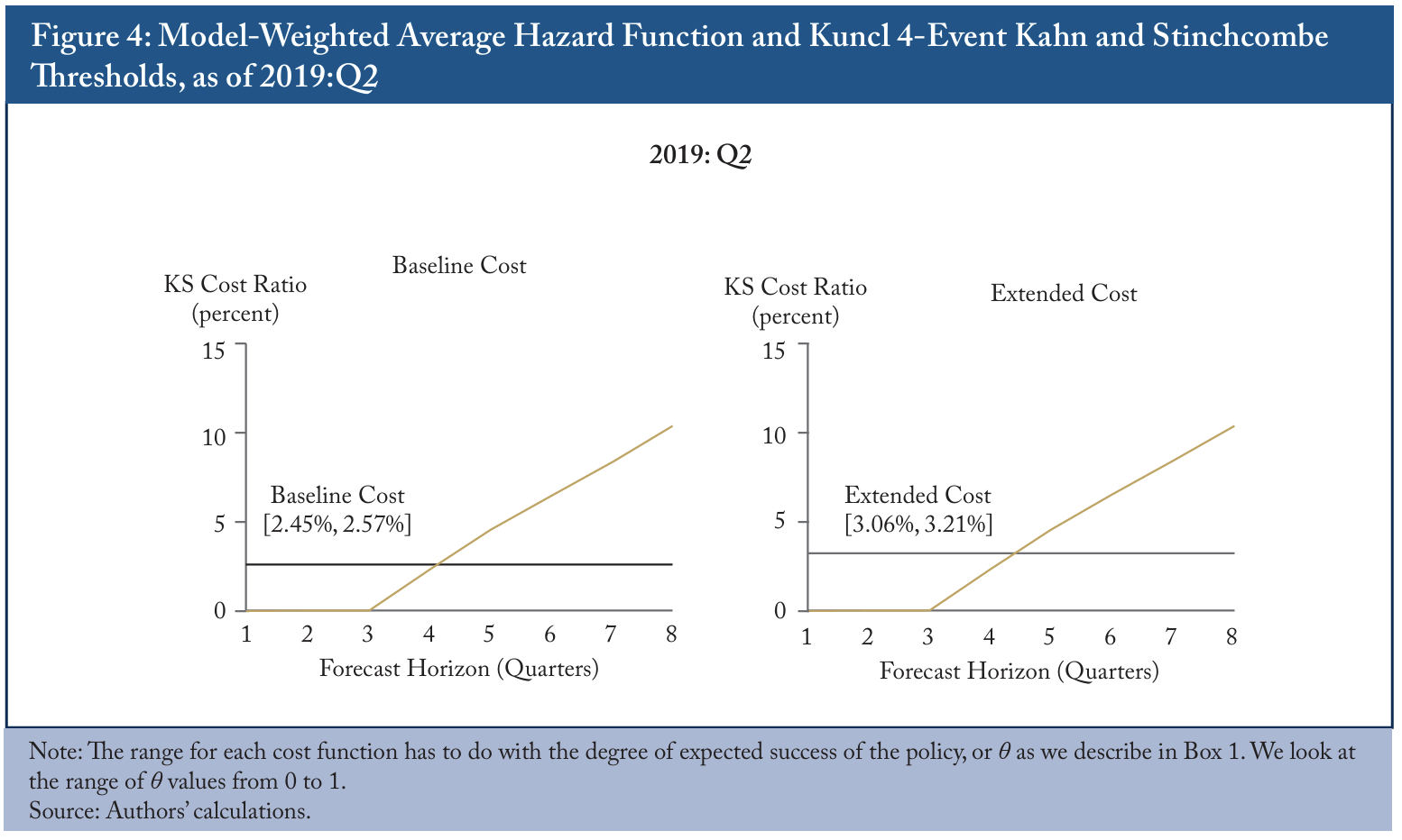
Based on this cost calibration, our policy framework suggests that, at mid-year 2019, the policymaker should not have considered taking action until the fourth projection quarter (mid2020), when the benefits of acting appear to outweigh the costs. We suggest instead that the policymaker continue monitoring conditions closely even if the chances of entering the low-financial stability state are low. Increases from this baseline cost calibration through the addition of forgone residential investment growth could modify the outcome of our analysis. However, as the extended cost in Figure 4 shows, the results change only marginally in that the hazard function does not intersect with the cost band until just after the fourth projection quarter - once again, mid-2020.

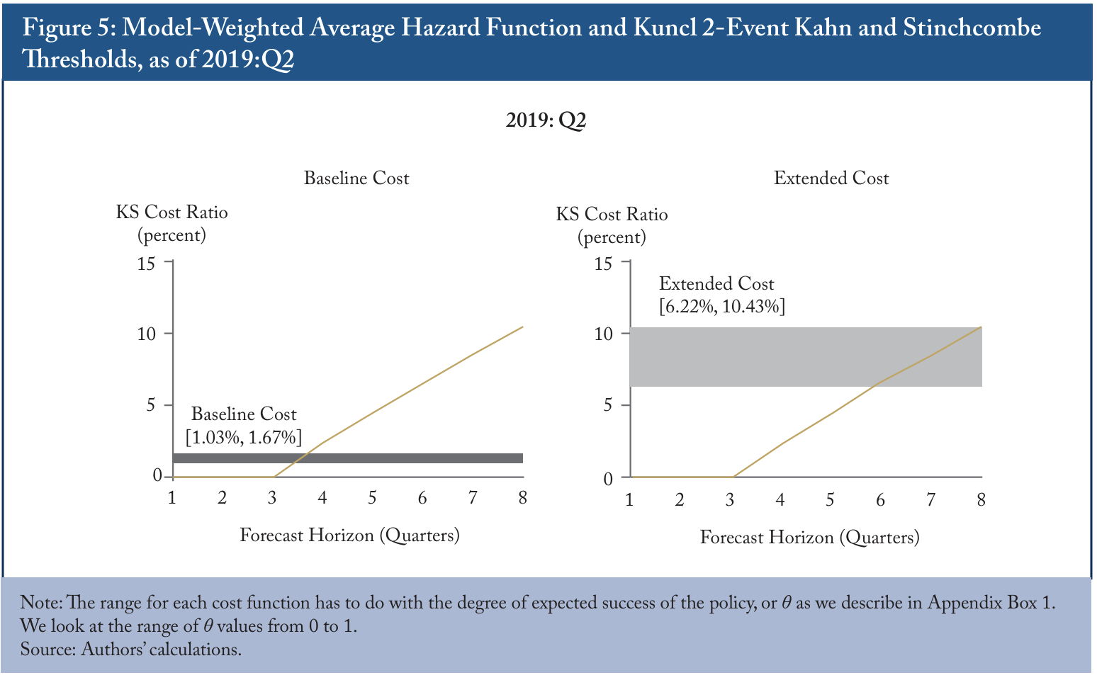
Figure 5 presents a slightly different policy recommendation based on a different data sample. As noted, the two policies enacted in March 2011 and July 2012 tightened LTV ratios and shortened maximum mortgage amortizations. They also are closer to our 2019:Q2 policy consideration date, and thus might provide a clearer perspective on current market conditions. This calibration also leaves out the anomalous data observed after the global financial crisis in 2008. The calibration lowers the cost band in the baseline cost panel in the graph, meaning that the hazard function intersects slightly earlier, between the third and fourth projection quarters, which corresponds roughly to the transition between the first and second quarters of 2020. The decline in residential investment growth is significant, however, suggesting major costs to the economy from enacting the policy. This higher cost suggests the need for greater care in the willingness to act in this extended-cost scenario (right panel). Accordingly, the hazard function now intersects the cost function in the sixth projection quarter – namely, the end of 2020. In this latter scenario, the calibration suggests that the policymaker defer action, since the costs of doing so are relatively high. Given the broader cost perspective provided by this cost measure, the more prudent recommendation to the policymaker then would have been no immediate action regarding these macroprudential (residential) mortgage policies was necessary.

As discussed earlier, we also want to look at the tightening of mortgage terms for first-time homebuyers as examined by Allen et al. (2017). Recall that the calibrated cost value of this policy is quite high, as it assumes that all first-time homebuyers who are affected by the tightening LTV ratio have no other way of accessing sufficient financing. Accordingly, as shown in Figure 6, even the lowest part of the cost range is above the 2019:Q2 hazard function over the entire projection horizon, which suggests that no policy action is necessary (dark shaded band). It is likely unreasonable, however, that all first-time homebuyers would be excluded from the market if the policy were enacted. Within our calibration framework, we can lower this exclusion assumption to examine when it might be reasonable to enact this policy. The two lighter-shaded lines in Figure 6 indicate how much lower the costs would have to be to warrant any policy action. We would have to assume that only 18 percent of first-time homebuyers are excluded to cause the policymaker to react within an eight-quarter forecast horizon, and only 8 percent are excluded for the policymaker to react within a five-quarter horizon. In our view, these exclusion rates are so unreasonably low that the policymaker should not consider taking the action at this time.

Conclusion

Macroprudential regulation has been on the rise since the 2007–09 global financial crisis. In Canada, the primary policy tools that have been employed in this regard are related to the residential housing market – namely, changes in mortgage loan-tovalue ratios and loan maturity requirements. In this Commentary, we have used the analytical framework developed by Brave and Lopez (2019) to forecast the probability of a state of low financial stability in the Canadian economy and to recommend when such a policy action might be taken in light of its costs and benefits.

We must abstract from the recent effects of COVID-19, as a global pandemic of this nature is near impossible for policymakers and regulators to predict. Our empirical analysis suggests that, as of the second quarter of 2019, and using data typically available to evaluate financial stability, the probability of a lengthy period of low financial stability is low. However, different calibrations of the costs and benefits of enacting a tightening of mortgage terms provide different perspectives on whether policymakers should act. Based on the methodology developed by Kahn and Stinchcombe (2015) for determining the optimal time for policy enactment and on calibration values from other recent Canadian policy studies, our results suggest that policymakers need not have acted at mid-year 2019, since the policy benefits would only have begun to accrue in late 2020. As such, our analysis suggests only a continued monitoring of mortgage market and financial stability conditions and further analysis of the structure of the policy tools available.

Appendix A: The Markov-Switching Model

We specify a univariate Markov-switching model, as per Hamilton (1989), capturing the joint dynamics of growth in real household spending and borrowing in order to identify distinct states of high and low stability for the Canadian mortgage market. We denote these states as {S+,S−}, respectively, and model the transitions between them based on changes in the joint dynamics of real household spending growth ∆ln(HHt ) and real growth in household borrowing ∆ln(Ct ).¹⁸18 We deflate both spending and borrowing by the Canadian CPI. This is in keeping with Giese et al. (2014), who find that real credit growth performs slightly better than nominal credit growth with respect to financial crisis signals. Our model, using data from 1990:Q1 through 2019:Q2, is specified as

where Yt = ∆ln(HHt ), Xt = {∆ln(HHt−1 ,∆ln(Ct ), ∆ln(Ct−1 ))}, and the state-dependent parameters are summarized in ΘS = {αS ,βS }. To differentiate between the states, we associate αS − < 0 with the low state, such that real household spending growth is negative on average when in this state.¹⁹19 Our specification differs slightly from that of Gadea Rivas and Perez-Quiros (2015) in that we do not restrict the effects of real credit growth in either state. As such, this allows for potentially richer joint dynamics within the two financial stability states. Note that Ajello et al. (2015) also use a contemporaneous credit growth variable in their specification of a crisis transition probability. The states of our model are assumed to follow a firstorder Markov process governed by the time-varying transition probability matrix Ωt , as per Diebold, Lee, and Weinbach (1994), such that

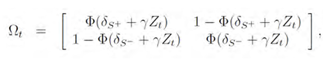
where Φ is the cumulative normal distribution and Zt represents an FSI variable. We introduce our four FSIs into Zt on an individual basis in order to limit the number of estimated parameters, and each is given a stationary transformation and standardized prior to estimation.²⁰20 We used log first differences for the house-price-to-rent and price-to-income ratios and household-credit-to-GDP and the four-quarter difference in the debt-servicing ratio. For our baseline model, we do not use an FSI and set the transition probabilities to be constant. Given the small number of transitions in our data, we also find it useful to follow Amisano and Fagan (2013) and require that the slope coefficients on Zt be common across the two states.²¹21 We used the Matlab MSREGRESS package of Perlin (2015) extended to the time-varying transition probability case by Ding (2012) for estimation, with 72 random initializations of each model used to pick the one that achieves the highest likelihood. For models with additional FSIs, we centered our initializations around the converged parameter estimates of our baseline model. For instances where convergence was first not achieved, we continued to draw random initializations until convergence. Correspondingly, our approach encompasses five model specifications. To arrive at a single characterization of the state of mortgage market stability, we combine these specifications using empirical Bayesian model averaging techniques as described in Clyde and George (2004). This framework weights each model by a measure of its fit of the data, giving more weight in relative terms to models that best capture the estimated transitions in the Canadian data; see Appendix B for further details.

Appendix B: Projecting Hazard Functions over the Policy Horizon

Based on the notation presented in Hamilton (2016), here we demonstrate the construction of the hazard functions needed for our pseudo outof-sample exercise. The relevant output from our Markov-switching models is the end-of-sample (T) transition probability matrix characterizing expected transitions between our financial stability states, summarized as

where is the estimated transition probability from state i at time T to state j at time T +1. To summarize the model-implied state, denote ξT as a (2×1) vector that uses a value of 1 to indicate the true, but unobservable, state, and 0 otherwise. For our estimated Markov-switching models, we generate

where the elements i = 1 corresponds to our high financial stability state S+, and i = 2 corresponds to our low financial stability state S−.

For forecasting purposes, define the matrix P whose (j,i) element corresponds to pij , such that each column sums to 1 – that is,

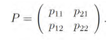
The one-step-ahead forecast of our modelimplied state is then E[ξT+1 |ξˆT ] = PξˆT , and the k-step-ahead forecast is E[ξT+k |ξˆT ] = PkξˆT . We generate forecasts in this manner for each of our five Markov-switching model specifications based on their estimates of ξˆT . We then use the forecast probabilities for each specification to construct vector probability forecasts for a defined adverse event of interest, which we denote as the conditional hazard function HT (k). Using the notation above,

which refers to the (2,1) element in the product for each value of k ϵ [1,5].²²22 For the time-varying probability models, the out-of-sample projections could be conditioned on projections for Zt+k. In the main text, we instead treat these variables as fixed at their end-of-sample values.

As noted in the main text, the usefulness of this event to a policymaker is likely limited. Therefore, we instead frame the policymaker’s problem as projecting out the hazard function at time T of experiencing four consecutive quarters of the low financial stability state S− over the eight-quarter forecast horizon. Note that the policymaker will have in hand the model-implied state probabilities of the three quarters leading up to the projection point T (that is, quarters T − 2 through T), which inform the probability of the four-quarter adverse event’s occurring in quarter T +1. With three conditional in-sample quarters and eight out-ofsample quarters over which to project, we have 2,048(= 211) state paths to consider. For each path, we determine the probability of the fourquarter adverse event’s occurring, and we then use the likelihood of each path to weight them in a corresponding four-quarter hazard function for each of our five model specifications.

To obtain a single hazard function for our policy exercise, we use our empirical Bayesian model averaging procedure, weighting each specification by a measure of its model fit. Defining the set of model specifications as Ξ, the posterior probability p(Ξm |Y,X,Z) assigned to each one of our m = 1,2,...,5 specifications is given by

where BIC(Ξm ) is the Bayesian Information Criterion and p(Ξm ) is a uniform prior.

Appendix C: Markov Regime-Switching Model Parameters

The transition probabilities are denoted by δ1 , the probability of remaining in the high stability state, and δ2 , the probability of transitioning from low stability to high stability and the effect of the FSIs on these probabilities (γFSI). The α and β parameter estimates indicate the co-movement of real household spending (HHSP) with real household borrowing growth and changes in the unemployment rate (UR) in our high (S+) and low (S−) stability states. We note that defining δ1 and δ2 the way we do is a result of how we set up the policy question. Specifically, implementing a macroprudential policy ideally occurs in a high financial stability state, and part of this decision requires a forecast of how long the economy is expected to be in the low financial stability state – that is, how quickly it gets back to the high financial stability state.

References

Ajello, A., T. Laubach, D. Lopez-Salido, and T. Nakata. 2015. “Financial Stability and Optimal Interest-Rate Policy.” Finance and Economics Discussion Series 2016-067. Washington, DC: Board of Governors of the Federal Reserve System.

Allen, J., T. Grieder, B. Peterson, and T. Roberts. 2017. “The Impact of Macroprudential Housing Finance Tools in Canada.” BIS Working Papers 632. Basel: Bank for International Settlements.

Amisano, G., and G. Fagan. 2013. “Money Growth and Inflation: A Regime Switching Approach.” International Journal of Money and Finance 33 (March): 118–45.

Bank of Canada. 2019. Financial System Review. May.

Bazelon, C., and K. Smetters. 1999. “Discounting Inside the Washington D.C. Beltway.” Journal of Economic Perspectives 13 (4): 213–28.

Bilyk, O., and M. Tenyenhuis. 2018. “The Impact of Recent Policy Changes on the Canadian Mortgage Market.” Bank of Canada Staff Analytical Note 2018-35. Ottawa: Bank of Canada.

Brave, S., and J. Lopez. 2019. “Calibrating Macroprudential Policy to Forecasts of Financial Stability.” International Journal of Central Banking 15 (1): 1–59.

Clyde, M., and E. I. George. 2004. “Model Uncertainty.” Statistical Science 19 (1): 81–94.

Diebold, F.X., J.-H. Lee, and G.C. Weinbach. 1994. “Regime Switching with Time-Varying Transition Probabilities.” In Nonstationary Time Series Analysis and Cointegration, ed. Colin P. Hargreaves, 283–302. Oxford: Oxford University Press.

Ding, Z. 2012. “An Implementation of Markov Regime Switching Model with Time Varying Transition Probabilities in MATLAB.” Manuscript.

Drehmann, M., and M. Juselius. 2013. “Evaluating Early Warning Indicators of Banking Crises: Satisfying Policy Requirements.” BIS Working Papers 421. Basel: Bank for International Settlements.

Drehmann, M., M. Juselius, and A. Korinek. 2017. “Accounting for Debt Service: The Painful Legacy of Credit Booms.” BIS Working Paper 645. Basel: Bank for International Settlements.

Duprey, T., and T. Roberts. 2017. “A Barometer of Canadian Financial System Vulnerabilities.” Bank of Canada Staff Analytical Note 2017-24. Ottawa: Bank of Canada.

Edge, R.M., and N. Liang. 2019. “New Financial Stability Governance Structures and Central Banks.” Federal Reserve Board, Finance and Economics Discussion Series, Working Paper 2019-019.

Gadea, Rivas, M.D., and G. Perez-Quiros. 2015. “The Failure to Predict the Great Recession – A View through the Role of Credit.” Journal of the European Economic Association 13 (3): 534–59.

Giese, J., H. Andersen, O. Bush, C. Castro, M. Farag, and S. Kapadia. 2014. “The Credit-to-GDP Gap and Complementary Indicators for Macroprudential Policy: Evidence from the U.K.” International Journal of Finance and Economics 19 (1): 25–47.

Hamilton, J.D. 1989. “A New Approach to the Economic Analysis of Nonstationary Time Series and the Business Cycle.” Econometrica 57 (2): 357–84.

———. 2016. “Macroeconomic Regimes and Regime Shifts.” NBER Working Paper 21863. Cambridge, MA: National Bureau of Economic Research.

IMF (International Monetary Fund). 2014a. Canada Financial Sector Stability Assessment. IMF Country Report 14/29. Washington, DC.: IMF. February.

———. 2014b. Canada Financial Sector Assessment Program. IMF Country Report 14/73. Washington, DC: IMF. March.

Khan, U., and M.B. Stinchcombe. 2015. “The Virtues of Hesitation: Optimal Timing in a Nonstationary World.” American Economic Review 105 (3): 114776.

Kronick, J. 2017. Spendthrifts and Savers: Are Canadians Acting Like They Are “House Poor” or “House Rich”? Commentary 482. Toronto: C.D. Howe Institute. June.

———. 2018. Productivity and the Financial Sector: What’s Missing? Commentary 508. Toronto: C.D. Howe Institute. April.

Kronick, J., and S. Ambler. 2020. Predicting Financial Crises: The Search for the Most Telling Red Flag in the Economy. Commentary 564. Toronto: C.D. Howe Institute. February.

Kuncl, M. 2016. “Assessment of the Effects of Macroprudential Tightening in Canada.” Bank of Canada Staff Analytical Note 2016-12. Ottawa: Bank of Canada.

Le Pan, N. 2017. Opportunities for Better Systemic Risk Management in Canada. Commentary 490. Toronto: C.D. Howe Institute. September.

Naglie, H. 2017. Not Ready for Prime Time: Canada’s Proposed New Securities Regulator. Commentary 489. Toronto: C.D. Howe Institute. September.

Perlin, M. 2015. “MS_Regress: The MATLAB Package for Markov Regime Switching Models.” Manuscript.

van Oodt, M.R.C. 2018. “Calibrating the Magnitude of the Countercyclical Capital Buffer using MarketBased Stress Tests.” Bank of Canada Staff Working Paper 2018-54. Ottawa: Bank of Canada.